Variogram models#
Parameters#
Variograms are set with set_vgm() using keyword arguments:
k.set_vgm(
    ivar=1, jvar=1,
    vtype="sph",
    nugget=0.05,
    sill=0.45,
    a_major=500.0,
    a_minor1=200.0,
    a_minor2=200.0,   # 3-D only; defaults to a_minor1
    azimuth=45.0,
    dip=0.0,
    plunge=0.0,
)
Parameter |
Default |
Description |
|---|---|---|
|
(required) |
Model type code (see table below) |
|
|
Nugget effect (discontinuity at origin) |
|
|
Partial sill — variance contributed by this structure |
|
|
Range along the major (longest) axis; see per-model meaning below |
|
|
Range along the first minor axis (defaults to isotropic) |
|
|
Range along the vertical axis (3-D only) |
|
|
Azimuth of major axis, degrees clockwise from North |
|
|
Dip angle of the major axis below horizontal, degrees positive downward |
|
|
Rotation of the semi-axes about the major axis, degrees |
|
|
|
|
|
|
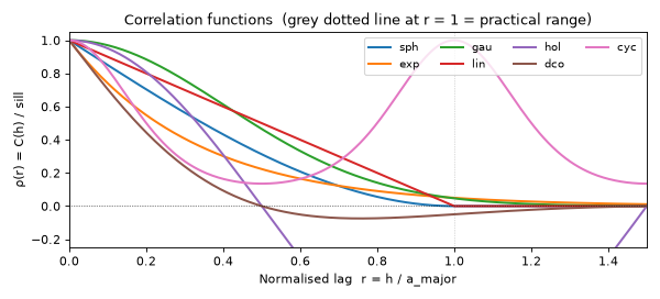
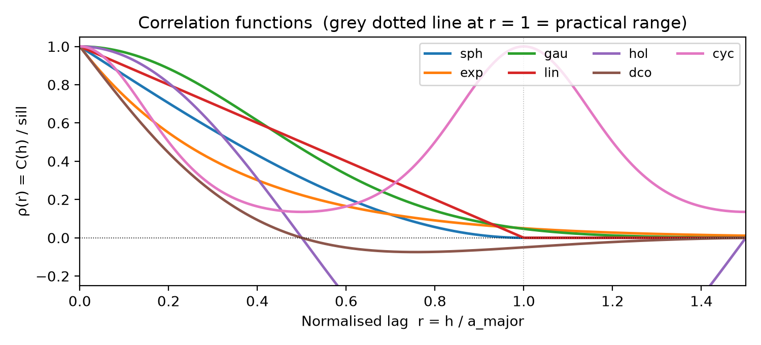
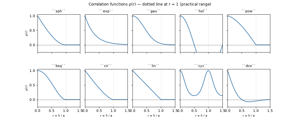
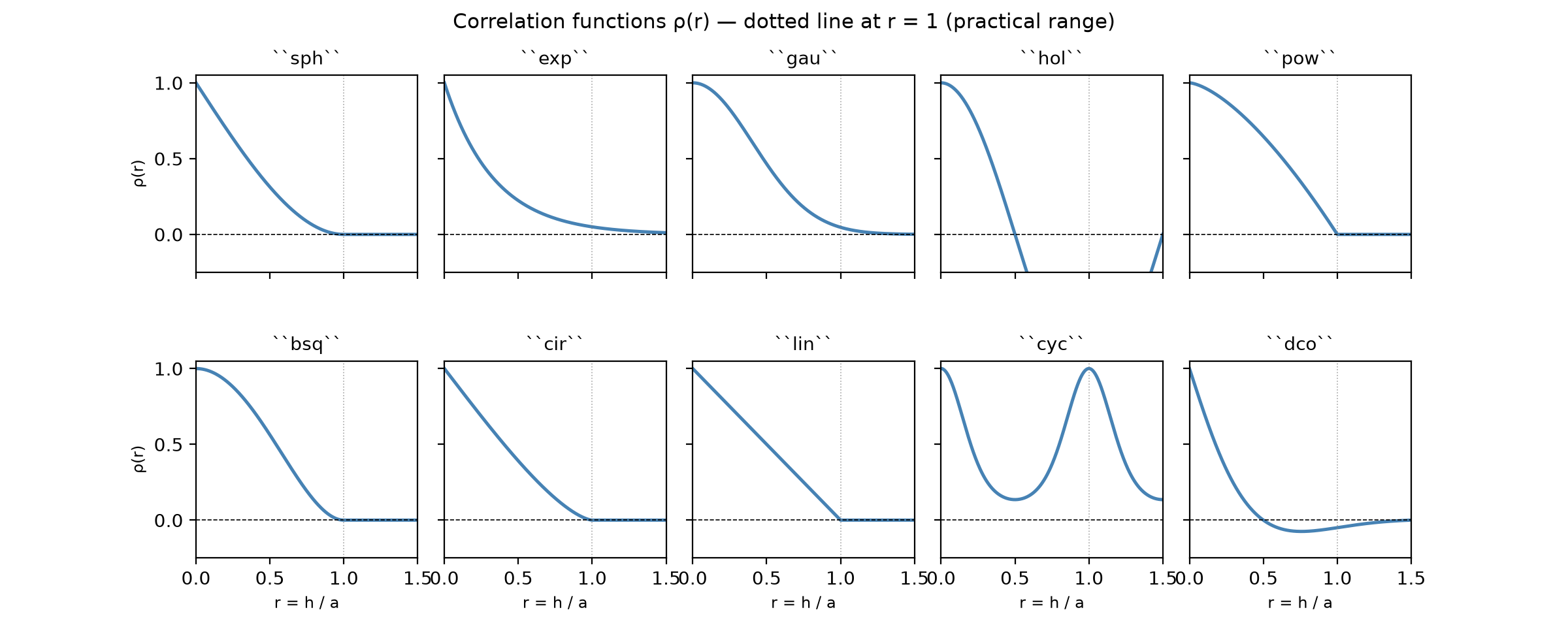
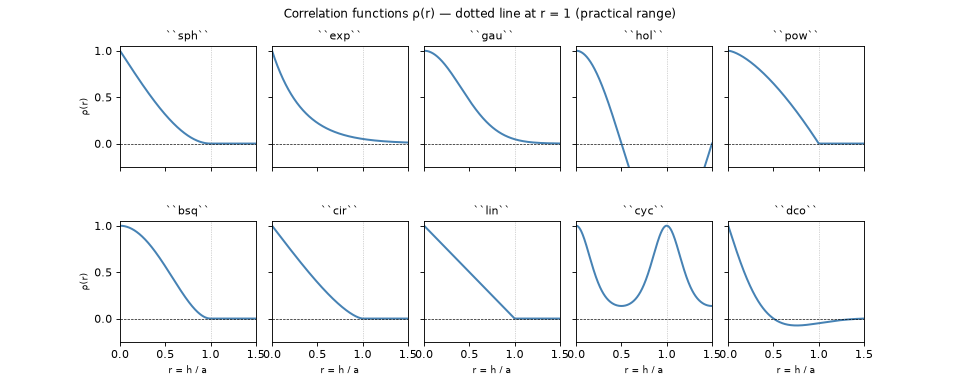
The dimensionless lag is \(r = h / a_\text{major}\) (after anisotropy scaling). The covariance is \(C(h) = \text{sill} \times \rho(r)\) where \(\rho(r)\) is the correlation function listed in the table below.
Supported model types#
Code |
Name |
Correlation \(\rho(r)\) |
|---|---|---|
|
Pure nugget |
\(0\) for \(r > 0\); 1 at origin |
|
Spherical |
\(1 - \tfrac{3}{2}r + \tfrac{1}{2}r^3\) for \(r < 1\), else \(0\) |
|
Exponential |
\(\exp(-3r)\) |
|
Gaussian |
\(\exp(-3.0625\,r^2)\) |
|
Hole effect |
\(\cos(\pi r)\) |
|
Power |
\(1 - r^{1.5}\) for \(r < 1\), else \(0\) |
|
Bi-square |
\((1 - r^2)^2\) for \(r < 1\), else \(0\) |
|
Circular |
\(1 - \tfrac{2}{\pi}\!\left(r\sqrt{1-r^2} + \arcsin r\right)\) for \(r < 1\), else \(0\) |
|
Linear |
\(1 - r\) for \(r < 1\), else \(0\) |
|
GP periodic |
\(\exp\!\left(-2\sin^2(\pi r)\right)\) |
|
Damped cosine |
\(\exp(-3r)\cos(\pi r)\) |
For sph, exp, and gau the practical range convention is used:
\(\rho(1) \approx 0\) (spherical reaches exactly 0; exponential and
Gaussian reach \(\approx 5\%\)), so a_major is the distance at which
spatial correlation is effectively zero.
Model notes#
Hole effect (hol)#
A pure cosine with period \(2a\). Correlation is zero at \(h = a/2\), reaches its most negative value (\(-\text{sill}\)) at \(h = a\), and returns to \(+\text{sill}\) at \(h = 2a\). Valid in 1-D and 2-D; use with caution in 3-D (not guaranteed positive-definite). The oscillation never damps, so the kriging matrix can be indefinite — the SSYTRF fallback solver handles this.
Damped cosine (dco)#
An oscillating covariance that decays exponentially with distance. ``a_major`` controls both the decay length and the oscillation period simultaneously — the first zero-crossing is at \(h = a/2\) and the first negative lobe peaks at \(h = a\). Valid and positive-definite in all dimensions. Suitable when the cyclic pattern weakens over long distances, e.g. annual signals in a climate record with increasing measurement gaps.
GP periodic / ExpSineSquared (cyc)#
``a_major`` is the period — correlation returns to sill at every
integer multiple of a_major. The model is always positive (correlation
\(\geq \exp(-2) \approx 0.14\) at the half-period \(h = a/2\)) and is
valid in all dimensions.
This is identical to the scikit-learn
ExpSineSquared
kernel with periodicity = a_major and length_scale = 1. The
length-scale (smoothness within each cycle) is fixed; only the period is a
free parameter.
Choosing between cyc and dco:
|
|
|
|---|---|---|
Cyclicity |
Strictly periodic — repeats forever |
Quasi-periodic — damps with distance |
|
Period of oscillation |
Decay length ≈ oscillation half-period |
Correlation at \(h = a/2\) |
\(\exp(-2) \approx 0.14\) |
\(0\) (first zero-crossing) |
Correlation at \(h = a\) |
\(1\) (full repeat) |
\(-\exp(-3) \approx -0.05\) |
Min correlation |
\(\exp(-2) > 0\) (always positive) |
Negative — can cause Cholesky failure |
Good for |
Annual cycles, tidal data, repeating spatial patterns |
Damped oscillations, waves losing energy with distance |
Single-structure model#
k.set_vgm(ivar=1, jvar=1,
          vtype="sph", nugget=0.05, sill=0.95, a_major=500.0)
Nested (multi-structure) model#
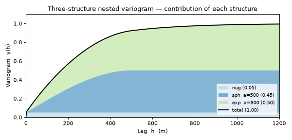
Call set_vgm multiple times. Each call appends one structure
(append=True is the default):
k.set_vgm(ivar=1, jvar=1, vtype="nug", nugget=0.05, sill=0.0,  a_major=1.0)
k.set_vgm(ivar=1, jvar=1, vtype="sph", nugget=0.0,  sill=0.45, a_major=500.0, a_minor1=200.0, azimuth=45.0)
k.set_vgm(ivar=1, jvar=1, vtype="exp", nugget=0.0,  sill=0.50, a_major=800.0)
# total sill = 0.05 + 0.45 + 0.50 = 1.0
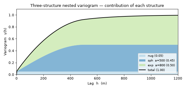
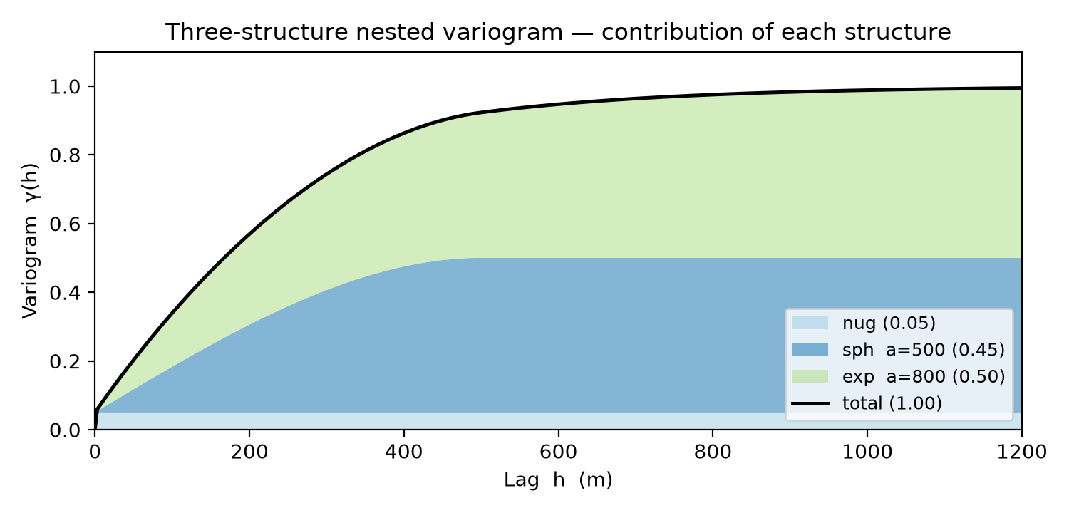
The variogram \(\gamma(h) = \text{sill} - C(h)\) for each structure stacks additively:
Periodic + background trend#
A common pattern for time-series data with an annual cycle and a long-range trend:
k.set_vgm(ivar=1, jvar=1, vtype="nug", nugget=0.1, sill=0.0,  a_major=1.0)
k.set_vgm(ivar=1, jvar=1, vtype="cyc", nugget=0.0, sill=0.6,  a_major=1.0)   # period = 1 year
k.set_vgm(ivar=1, jvar=1, vtype="exp", nugget=0.0, sill=0.3,  a_major=5.0)   # long-range decay
Python-side model object#
For variogram analysis, fitting, and plotting, use
krigekit.variogram.VariogramModel to build the same structure list in
Python before applying it to a Kriging object:
from krigekit import Kriging, VariogramModel

model = VariogramModel()
model.set_vgm(vtype="nug", nugget=0.05, sill=0.0, a_major=1.0)
model.set_vgm(vtype="sph", nugget=0.0, sill=0.45, a_major=500.0)
model.set_vgm(vtype="exp", nugget=0.0, sill=0.50, a_major=800.0)

gamma = model.variogram(h)
cov   = model.covariance(h)

k = Kriging()
k.set_obs(ivar=1, coord=obs_coord, value=obs_value)
model.apply_to(k, ivar=1, jvar=1)
VariogramModel.set_vgm uses the same keyword names as
Kriging.set_vgm except that ivar and jvar are omitted. Use
to_kriging_specs() if you want the list of dictionaries instead:
for spec in model.to_kriging_specs(replace=True):
    k.set_vgm(ivar=1, jvar=1, **spec)
Product structures are represented the same way. A structure with
product=True is multiplied with the immediately preceding structure in
covariance space:
model = VariogramModel()
model.set_vgm(vtype="exp", sill=1.0, a_major=5.0)
model.set_vgm(vtype="hol", sill=1.0, a_major=1.0, product=True)
# C(h) = C_exp(h; a=5) * C_hol(h; a=1)
The fitting helper can use the same structure template. Pass
return_model=True to receive a fitted VariogramModel:
from krigekit.variogram import fit_vgm

p, pcov, fitted = fit_vgm(
    avg_vgm_table,
    models=(
        {"vtype": "exp"},
        {"vtype": "hol", "product": True},
    ),
    p0=(1.0, 5.0, 1.0, 1.0),  # sill/range for each structure
    return_model=True,
)

fitted.apply_to(k, ivar=1, jvar=1)
The object method is a shorter form when you already have a model template. It can fit an averaged variogram table directly:
model = VariogramModel()
model.set_vgm(vtype="sph", nugget=0.05, sill=0.95, a_major=500.0)

fitted, pcov = model.fit(avg_vgm_table)
fitted.apply_to(k, ivar=1, jvar=1)
Or let the model compute the empirical and averaged variogram from stored observations:
model = VariogramModel()
model.set_obs(obs_coord, obs_value)
model.set_vgm(vtype="sph", nugget=0.05, sill=0.95, a_major=500.0)

fitted, pcov = model.fit(
    raw_kwargs={"cutoff": 2000.0, "calc_angle": True, "verbose": False},
    avg_kwargs={"h_width": 100.0},
)
For weighted fitting, use weight_col or weights. Larger weights have
more influence; for averaged variograms, the bin pair count is often a useful
starting point:
fitted, pcov = model.fit(weight_col=("variogram", "count"))
Alternatively, pass sigma_col for SciPy-style standard deviations. Do not
pass sigma_col and weights at the same time.
After fitting, parameters can be adjusted manually without rebuilding the
object. set_params() uses the same flat convention as fit():
model.fit(inplace=True)
model.set_params([0.12, 5000.0, 0.02])  # sill, range, nugget
model.plot()
For structure fields outside the flat fitting vector, such as anisotropy, use
set_structure_params():
model.set_structure_params(0, a_minor1=2500.0, azimuth=35.0)
For a nested model where all structures share the same orientation and
minor/major ratio, set_anisotropy() is shorter:
model.set_anisotropy(anis1=0.16, azimuth=90.0)
If the orientation is known but the major and minor ranges should be fitted,
average the empirical cloud along the fixed model axes and use
fit_anisotropy():
model.set_vgm(vtype="sph", sill=0.8, a_major=1000.0,
              a_minor1=300.0, azimuth=90.0)
model.calc_experimental(cutoff=3000.0, calc_angle=True, verbose=False)
directional = model.calc_directional_average(
    h_width=100.0,
    cutoff=2500.0,
    angle_tol=15.0,
)
model.fit_anisotropy(
    directional,
    p0=(0.8, 1000.0, 300.0, 0.05),
    weight_col="count",
    inplace=True,
)
fit() remains the ordinary one-dimensional lag fit with flat parameters
sill, a_major, ..., nugget. fit_anisotropy() keeps azimuth,
dip and plunge fixed and fits sill, a_major, a_minor1 for each
structure, plus a_minor2 for 3-D directional fits.
For 3-D fits, the shortest axis (a_minor2) is usually the hardest
parameter to estimate. Prefer h_bins with h_width=None so
calc_directional_average() computes a separate effective bin width for
each axis. This gives the short axis narrower lag bins instead of forcing it
to share a coarse major-axis bin width:
directional = model.calc_directional_average(
    h_bins=18,
    cutoff=36.0,
    angle_tol=20.0,
)
Raw pair-count weights can also let the major and minor1 curves dominate
the least-squares objective. Normalize counts within each axis before fitting
to give a_minor2 comparable influence:
directional["axis_weight"] = (
    directional["count"]
    / directional.groupby("axis", observed=True)["count"].transform("sum")
)
model.fit_anisotropy(
    directional,
    include_minor2=True,
    fit_nugget=False,
    weight_col="axis_weight",
    inplace=True,
)
The preferred verb-style names for new code are calc_experimental() and
calc_average():
raw = model.calc_experimental(cutoff=2000.0, verbose=False)
avg = model.calc_average(h_width=100.0)
These calls cache workflow state on the model. The raw cloud, averaged table,
fitted parameter vector, and fitted covariance are available as _raw,
_avg, _params, and _pcov; sklearn-style aliases
raw_variogram_, avg_variogram_, params_, and pcov_ are also
provided for user-facing access.
plot() draws the cached averaged variogram and the current model curve:
model.plot()
plot_map() draws the cached raw variogram cloud as a 2-D variogram map.
By default it overlays the first structure’s azimuth and anisotropy ellipse,
which is useful for checking whether the chosen direction agrees with the
experimental cloud before calling fit_anisotropy():
model.calc_experimental(cutoff=3000.0, calc_angle=True, verbose=False)
model.plot_map(cutoff=2500.0)
model.plot_map(angle_aniso="estimate", cutoff=2500.0)
For 3-D clouds, plot_map3d() draws a horizontal lag slice and a vertical
fence aligned with the model or estimated major azimuth. The raw cloud must
include lag angles:
model.calc_experimental(cutoff=3000.0, calc_angle=True, verbose=False)
model.plot_map3d(cutoff=2500.0)
model.plot_map3d(angle_aniso="estimate", cutoff=2500.0)
model.plot_map3d(cutoff=2500.0, fill_nan=True)  # display-only in-range smoothing
variogram(h) and covariance(h) evaluate a lag-distance curve. To
evaluate between coordinates with anisotropy applied, use
calc_variogram() or calc_covariance():
gamma = model.calc_variogram([0.0, 0.0], [500.0, 250.0])
covmat = model.calc_covariance(obs_coord, grid_coord, pairwise=True)
Multivariable variogram systems#
Use VariogramSystem when a cokriging workflow needs observations and
models for several variables. The API mirrors the kriging object by carrying
ivar and jvar through set_obs() and set_vgm():
from krigekit import Kriging, VariogramSystem

system = VariogramSystem(nvar=2)
system.set_obs(ivar=1, coord=coord_v, value=value_v)
system.set_obs(ivar=2, coord=coord_u, value=value_u)

system.set_vgm(ivar=1, jvar=1, vtype="sph", sill=1.0, a_major=500.0)
system.set_vgm(ivar=2, jvar=2, vtype="sph", sill=0.6, a_major=500.0)
system.set_vgm(ivar=1, jvar=2, vtype="sph", sill=0.4, a_major=500.0)

system.calc_experimental(ivar=1, jvar=1, cutoff=2000.0, verbose=False)
system.calc_experimental(ivar=2, jvar=2, cutoff=2000.0, verbose=False)
system.calc_experimental(ivar=1, jvar=2, cutoff=2000.0, verbose=False)
system.calc_average(h_width=100.0)
For cross pairs, calc_experimental(ivar, jvar) uses the traditional LMC
cross-variogram estimator when the two variables are collocated:
If the variables are heterotopic, set cross="pseudo" explicitly to use the
older pseudo cross-cloud based on all between-variable pairs. Do not interpret
that pseudo sill as an LMC cross-sill.
fit_pair() fits a single pair independently. For cokriging, prefer
fit_lmc() because it fits all requested pairs together while enforcing a
positive-semidefinite sill matrix for each nested structure:
fitted_system, result = system.fit_lmc(
    fit_ranges=True,
    fit_nugget=True,
)

k = Kriging(nvar=2)
fitted_system.apply_to(k)
Product variogram (non-additive nesting)#
Setting product=True on a set_vgm call multiplies the new
structure with the immediately preceding one instead of adding it. The
Schur product
of two positive-definite covariance functions is always positive-definite, so
validity is guaranteed regardless of the parameter values chosen.
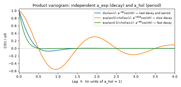
The primary use case is independent control over the decay envelope and the
oscillation period — something dco cannot provide because it ties both
to the same a_major:
# dco: decay length AND period both governed by a_major
k.set_vgm(1, 1, vtype="dco", sill=1.0, a_major=1.0)
# C(h) = exp(-3h) cos(πh)  — first zero at h = 0.5, coupled to range

# Product exp × hol: independent ranges
k.set_vgm(1, 1, vtype="exp", sill=1.0, a_major=5.0)                 # slow decay envelope
k.set_vgm(1, 1, vtype="hol", sill=1.0, a_major=1.0, product=True)  # oscillation half-period = 1
# C(h) = exp(-3h/5) cos(πh)  — same period as dco(a=1), but envelope decays 5× more slowly
Rules for product structures:
product=Trueon structure k multiplies with structure k−1.Both structures may have different
a_majorvalues (independent scales) but must share the same orientation (azimuth,dip,plunge).Chaining three or more consecutive
product=Truestructures multiplies left-to-right: A × B × C.To add a second independent product group, place a non-product structure between the two groups.
Weak periodic modulation#
A pure decay-times-periodic product makes the periodic kernel control the full covariance amplitude. For a weaker seasonal signal, add a non-periodic background group and give the product group a smaller sill:
with \(0 < B \ll A\). For annual data measured in years:
temporal = VariogramModel()
temporal.set_vgm("gau", nugget=3.4, sill=38.5, a_major=34.6)
temporal.set_vgm("gau", sill=2.6, a_major=34.6)
temporal.set_vgm("hol", sill=1.0, a_major=0.5, product=True)

temporal.apply_temporal_to(k, ivar=1, jvar=1)
The hol period is 2 * a_major, so a_major=0.5 is one year.
SpaceTimeKriging.set_vgm_temporal accepts the same product=True
semantics for temporal marginal structures.
Anisotropic model#
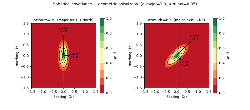
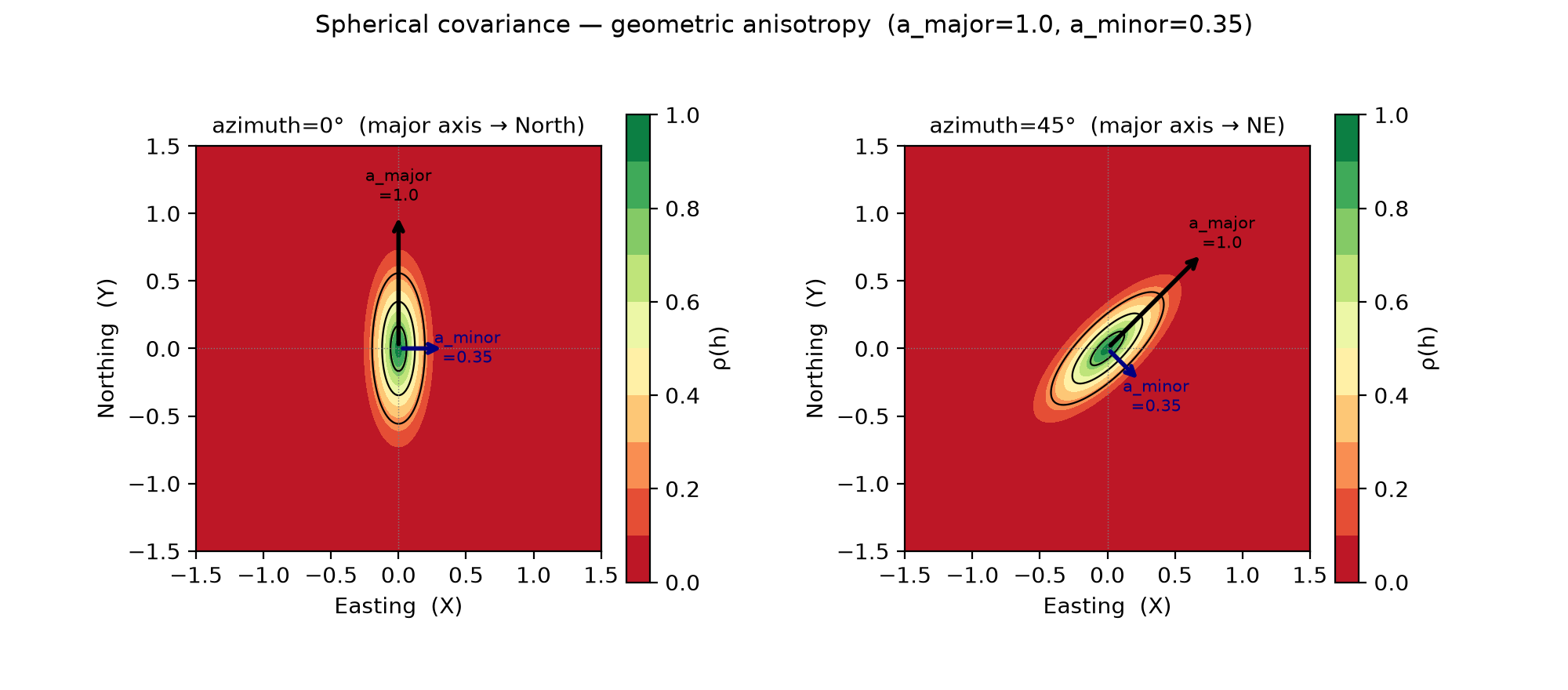
The rotation convention follows standard geostatistical practice:
azimuth: clockwise from North (Y-axis), in the XY plane
dip: tilt of the major axis below horizontal (positive downward)
plunge: rotation of the semi-axes around the major axis
a_major: range along the major (longest) axis
a_minor1: range perpendicular to major in the horizontal plane
a_minor2: range in the vertical direction (3-D)
At azimuth=0, dip=0, plunge=0 the major axis points North (Y direction).
k.set_vgm(ivar=1, jvar=1,
          vtype="sph",
          nugget=0.0, sill=1.0,
          a_major=1000.0, a_minor1=400.0,  # 2-D anisotropy
          azimuth=45.0)                     # major axis points NE
For 3-D add a_minor2 (vertical range) and dip / plunge.
Replacing a variogram on a reused object#
When reusing a Kriging object with a different variogram, pass
append=False on the first set_vgm call to clear the previous model:
# first run
k.set_obs(...)
k.set_vgm(ivar=1, jvar=1, vtype="sph", sill=1.0, a_major=500.0)
k.set_grid(...)
k.set_search(ivar=1)
k.solve()

# second run — different variogram
k.set_vgm(ivar=1, jvar=1, vtype="exp", sill=1.0, a_major=800.0, append=False)
k.solve()
Without append=False the second run would accumulate structures from the
first run, silently doubling (or tripling) the total sill.
Linear Model of Coregionalisation (LMC)#
For co-kriging with variables 1 and 2, every nested structure k must satisfy the LMC constraint:
where b denotes the partial sill for each variable pair. Violating this makes the co-kriging matrix indefinite and will produce negative variances.
The correlation coefficient per structure is:
A safe starting point is b12 = 0.8 * sqrt(b11 * b22) (ρ = 0.8).
Example LMC:
rho = 0.8
b11, b22 = 0.7, 0.3
b12 = rho * (b11 * b22) ** 0.5

k.set_vgm(ivar=1, jvar=1, vtype="sph", nugget=0.0, sill=b11, a_major=1000.0, a_minor1=500.0)
k.set_vgm(ivar=2, jvar=2, vtype="sph", nugget=0.0, sill=b22, a_major=1000.0, a_minor1=500.0)
k.set_vgm(ivar=1, jvar=2, vtype="sph", nugget=0.0, sill=b12, a_major=1000.0, a_minor1=500.0)