Space-time kriging of groundwater levels with a quasi-periodic covariance

This example fits spatial and temporal marginal variograms to obs_gwlevel.csv and then space-time kriges groundwater levels: well hydrographs with uncertainty bands, leave-one-well-out reconstruction of sparse wells, and a snapshot map validated against a holdout. The temporal marginal combines a slowly decaying long-term trend with a weak annual cycle, built as a multiplicative (product) covariance — a capability that lets krigekit represent quasi-periodic correlation with a provably valid model.

The data contain repeated groundwater-level measurements at 988 wells from 1978 through 2022, mostly at half-year or one-year intervals.

Data source. Groundwater-level measurements for the Middle Republican Natural Resources District (Middle Republican River basin, Nebraska), from the University of Nebraska–Lincoln Conservation and Survey Division statewide groundwater-level database (https://csd.unl.edu/water/groundwater/NebGW_Levels). Coordinates and ground elevation (dem10) are in feet; sl_lev_va is the measured groundwater level (head). Used here for non-commercial research and illustration; consult the CSD site for the current data and terms of use.

The two marginals need different pair definitions:

• The spatial variogram uses the long-term mean depth to water at each sufficiently sampled well. Depth to water is dem10 - sl_lev_va; this removes the broad topographic trend present in raw hydraulic head.

• The temporal variogram uses pairs from the same well only. Mixing different wells would fold the spatial gradient into the temporal marginal.

Note

For the integrated automatic fitting workflow, see examples/variogram/st_variogram_fitting_gwlevel.py. It uses VariogramModel for each marginal and SpaceTimeVariogramModel for the full lag surface and sum-metric coupling. This space-time kriging example keeps the marginal calculations and temporal parameter fit separate and explicit so the spatial, long-term temporal, and annual product-covariance contributions are easier to examine. The companion example also fits a nonzero sum-metric coupling term from the full space-time lag surface. This script retains a zero joint sill intentionally to isolate the marginal and annual-cycle behavior in the later comparisons.

The temporal covariance combines a smooth long-term Gaussian decay with a smaller annually periodic term:

\[C_T(h) = A\,G(h; a_T) + B\,G(h; a_T)\cos(2\pi h),\]

where \(G(h; a_T)=\exp[-3.0625(h/a_T)^2]\). Therefore,

\[\gamma_T(h) = \eta + A[1-G(h; a_T)] + B[1-G(h; a_T)\cos(2\pi h)].\]

This is a valid sum of covariance groups. In krigekit it is represented as one additive Gaussian structure plus a second Gaussian structure multiplied by a hole-effect structure. The hole-effect range is fixed at 0.5 years because its covariance is \(\cos(\pi h/a)\) and its period is 2*a.

from pathlib import Path

import matplotlib.pyplot as plt
import numpy as np
import pandas as pd
from scipy.optimize import least_squares
from scipy.spatial import Delaunay

from krigekit import Kriging, SpaceTimeKriging, VariogramModel


def _find_data_dir():
    """Locate test_data when run as a script or through Sphinx-Gallery."""
    candidates = []
    if "__file__" in globals():
        candidates.append(Path(__file__).resolve().parents[2] / "test_data")
    cwd = Path.cwd().resolve()
    candidates.extend([
        cwd / "test_data",
        cwd.parent / "test_data",
        cwd.parent.parent / "test_data",
    ])
    for candidate in candidates:
        if candidate.exists():
            return candidate
    raise FileNotFoundError("Could not locate the test_data directory.")


def _within_well_temporal_cloud(data, cutoff):
    """Return temporal lags and semivariances for pairs within each well."""
    frames = []
    for _, group in data.groupby("WellID", sort=False):
        if len(group) < 2:
            continue
        time = group["timeindex"].to_numpy(dtype=float)
        value = group["depth_to_water"].to_numpy(dtype=float)
        i, j = np.triu_indices(len(group), k=1)
        lag = np.abs(time[i] - time[j])
        keep = (lag > 0.0) & (lag <= cutoff)
        frames.append(pd.DataFrame({
            "distance": lag[keep],
            "variogram": 0.5 * (value[i[keep]] - value[j[keep]]) ** 2,
        }))
    return pd.concat(frames, ignore_index=True)


DATA_DIR = _find_data_dir()
SPATIAL_CUTOFF = 120_000.0
SPATIAL_WIDTH = 5_000.0
TEMPORAL_CUTOFF = 20.0
TEMPORAL_WIDTH = 0.5
MIN_WELL_OBS = 10

data = pd.read_csv(DATA_DIR / "obs_gwlevel.csv")
data["depth_to_water"] = data["dem10"] - data["sl_lev_va"]

print(
    f"{len(data):,} observations, {data['WellID'].nunique():,} wells, "
    f"{data['timeindex'].min():.1f}-{data['timeindex'].max():.1f}"
)

23,075 observations, 988 wells, 1978.0-2022.0

Fit the spatial marginal

A long-term mean is more stable than selecting one survey date, and requiring at least ten observations prevents short records from adding noisy well means.

The companion st_variogram_fitting_gwlevel.py example performs the marginal fits with VariogramModel and the joint fit with SpaceTimeVariogramModel. The calculations remain visible here to keep the focus on how separately estimated spatial and temporal components form the later space-time covariance.

well_mean = (
    data.groupby("WellID")
    .agg(
        x=("x", "first"),
        y=("y", "first"),
        depth=("depth_to_water", "mean"),
        count=("depth_to_water", "size"),
    )
    .query("count >= @MIN_WELL_OBS")
)

spatial = VariogramModel()
spatial.set_obs(
    well_mean[["x", "y"]].to_numpy(dtype=float),
    well_mean["depth"].to_numpy(dtype=float),
)
spatial.set_vgm(
    vtype="sph",
    nugget=50.0,
    sill=3_400.0,
    a_major=100_000.0,
)
spatial.calc_experimental(cutoff=SPATIAL_CUTOFF, verbose=False)
spatial.calc_average(h_width=SPATIAL_WIDTH)
spatial.fit(
    p0=(3_400.0, 100_000.0, 50.0),
    bounds=(
        (0.0, 1_000.0, 0.0),
        (10_000.0, 300_000.0, 1_000.0),
    ),
    weight_col=("variogram", "count"),
    inplace=True,
)

spatial_spec = spatial.to_kriging_specs()[0]
print(
    "Spatial spherical fit: "
    f"nugget={spatial_spec['nugget']:.1f}, "
    f"sill={spatial_spec['sill']:.1f}, "
    f"range={spatial_spec['a_major']:.0f} ft"
)

Spatial spherical fit: nugget=0.0, sill=3518.8, range=102013 ft

Calculate the temporal marginal

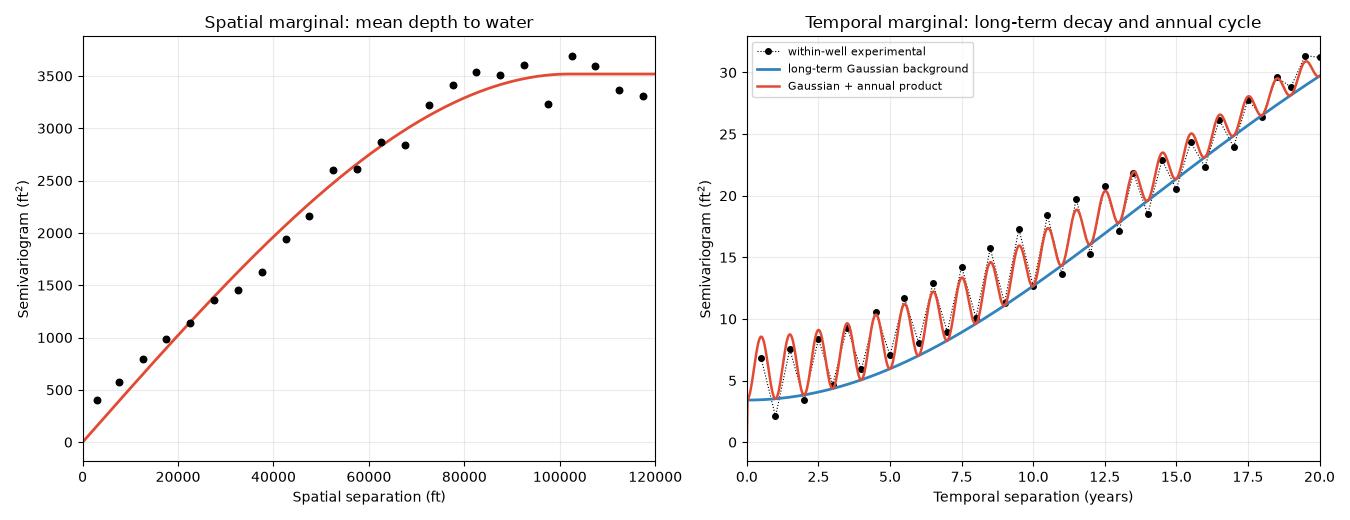
Only within-well pairs are admissible. With a 0.5-year bin width, integer lags compare the same sampling season while half-integer lags compare opposite seasons; the alternating semivariance is the annual signal.

temporal_cloud = _within_well_temporal_cloud(data, TEMPORAL_CUTOFF)
temporal_cloud["lag_bin"] = (
    temporal_cloud["distance"] / TEMPORAL_WIDTH + 1.0e-9
).astype(int)
temporal_avg = (
    temporal_cloud.groupby("lag_bin")
    .agg(
        distance=("distance", "mean"),
        variogram=("variogram", "mean"),
        count=("variogram", "size"),
    )
    .query("count >= 30")
    .reset_index(drop=True)
)

Fit long-term decay and annual covariance

The annual period is known from the sampling cycle, so it is fixed at one year. The fit estimates the nugget, background sill A, seasonal sill B, and the shared Gaussian practical range. Sharing the range makes the seasonal amplitude decay with the same long-term envelope.

Note

The fitted Gaussian range (~35 yr) is longer than the lag window used to estimate it (TEMPORAL_CUTOFF = 20 yr), so the long-term decay is only weakly constrained: within-well pairs at multi-decade lags are scarce, and the fit is governed mainly by the near-origin behaviour. The 44-year record is too short to pin down the multi-year decay precisely — a longer record would be needed to test it. This does not affect the demonstration: the annual product term and the spatial marginal drive the predictions, and over the 20-year window of interest the background covariance is effectively a slowly varying trend regardless of the exact range.

lag = temporal_avg["distance"].to_numpy()
gamma = temporal_avg["variogram"].to_numpy()
weight = np.sqrt(
    temporal_avg["count"].to_numpy()
    / temporal_avg["count"].max()
)


def temporal_variogram(params, h):
    """Evaluate the constrained Gaussian plus annual product model."""
    nugget, background_sill, seasonal_sill, decay_range = params
    decay = np.exp(-3.0625 * (np.asarray(h) / decay_range) ** 2)
    annual = np.cos(2.0 * np.pi * np.asarray(h))
    return (
        nugget
        + background_sill * (1.0 - decay)
        + seasonal_sill * (1.0 - decay * annual)
    )


fit = least_squares(
    lambda params: weight * (temporal_variogram(params, lag) - gamma),
    x0=(4.0, 35.0, 2.5, 30.0),
    bounds=(
        (0.0, 0.0, 0.0, 1.0),
        (50.0, 100.0, 20.0, 100.0),
    ),
)
nugget_t, background_sill, seasonal_sill, decay_range = fit.x

temporal = VariogramModel()
temporal.set_vgm(
    vtype="gau",
    nugget=nugget_t,
    sill=background_sill,
    a_major=decay_range,
)
temporal.set_vgm(
    vtype="gau",
    sill=seasonal_sill,
    a_major=decay_range,
)
temporal.set_vgm(
    vtype="hol",
    sill=1.0,
    a_major=0.5,
    product=True,
)

np.testing.assert_allclose(
    temporal.variogram(lag),
    temporal_variogram(fit.x, lag),
    rtol=1.0e-12,
    atol=1.0e-12,
)

# Background-only temporal model: a single Gaussian with the SAME total sill and
# range but no annual product term.  Used later to isolate the contribution of
# the multiplicative (quasi-periodic) structure at equal temporal variance.
temporal_background = VariogramModel()
temporal_background.set_vgm(
    vtype="gau",
    nugget=nugget_t,
    sill=background_sill + seasonal_sill,
    a_major=decay_range,
)

print(
    "Temporal fit: "
    f"nugget={nugget_t:.2f}, background sill={background_sill:.2f}, "
    f"seasonal sill={seasonal_sill:.2f}, "
    f"Gaussian range={decay_range:.2f} yr, annual period=1 yr"
)
print("Temporal SpaceTimeKriging specs:")
for spec in temporal.to_temporal_specs():
    print(f"  {spec}")

Temporal fit: nugget=3.42, background sill=38.52, seasonal sill=2.56, Gaussian range=34.63 yr, annual period=1 yr
Temporal SpaceTimeKriging specs:
  {'vtype': 'gau', 'nugget': 3.416256944421214, 'sill': 38.51793354068589, 'at_k': 34.625347061395054, 'product': False}
  {'vtype': 'gau', 'nugget': 0.0, 'sill': 2.562483076603054, 'at_k': 34.625347061395054, 'product': False}
  {'vtype': 'hol', 'nugget': 0.0, 'sill': 1.0, 'at_k': 0.5, 'product': True}

Plot the fitted marginals

The blue temporal curve is the non-seasonal background. The red curve is the complete valid product model; its alternating half-year response weakens as the Gaussian covariance envelope decays.

fig, axes = plt.subplots(1, 2, figsize=(13.5, 5.2))

spatial_avg = spatial.avg_variogram_
h_space = np.linspace(0.0, SPATIAL_CUTOFF, 400)
axes[0].scatter(
    spatial_avg[("distance", "mean")],
    spatial_avg[("variogram", "mean")],
    c="black",
    s=22,
    label="experimental",
    zorder=3,
)
axes[0].plot(h_space, spatial.variogram(h_space), color="#e34a33", lw=2.0)
axes[0].set(
    xlabel="Spatial separation (ft)",
    ylabel=r"Semivariogram (ft$^2$)",
    title="Spatial marginal: mean depth to water",
    xlim=(0.0, SPATIAL_CUTOFF),
)

h_time = np.linspace(0.0, TEMPORAL_CUTOFF, 800)
background = (
    nugget_t
    + (background_sill + seasonal_sill)
    * (1.0 - np.exp(-3.0625 * (h_time / decay_range) ** 2))
)
axes[1].plot(
    temporal_avg["distance"],
    temporal_avg["variogram"],
    color="black",
    marker="o",
    ms=4,
    lw=0.8,
    ls=":",
    label="within-well experimental",
)
axes[1].plot(
    h_time,
    background,
    color="#3182bd",
    lw=2.0,
    label="long-term Gaussian background",
)
axes[1].plot(
    h_time,
    temporal.variogram(h_time),
    color="#e34a33",
    lw=1.8,
    label="Gaussian + annual product",
)
axes[1].set(
    xlabel="Temporal separation (years)",
    ylabel=r"Semivariogram (ft$^2$)",
    title="Temporal marginal: long-term decay and annual cycle",
    xlim=(0.0, TEMPORAL_CUTOFF),
)
axes[1].legend(fontsize=8)

for ax in axes:
    ax.grid(alpha=0.25)

fig.tight_layout()
plt.show()

Krige time series at two wells

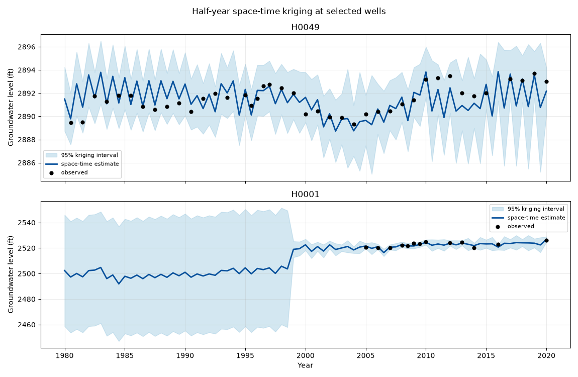
Predict at half-year intervals from 1980 through 2020 for H0049 and H0001. All observations are retained, so this is a conditional interpolation and smoothing exercise rather than leave-one-well-out validation. H0049 has a dense record over most of the interval. H0001 begins in 2005, so its earlier values are reconstructed from surrounding wells.

The spatial and temporal marginals are combined additively with a zero joint sill. This matches the fitted decomposition into a persistent spatial depth-to-water field and a smaller temporal departure:

\[C(\mathbf{h}, u) = C_S(\mathbf{h}) + C_T(u).\]

time_at affects neighbour search, not this covariance equation. The ratio of fitted practical ranges converts one year into an equivalent spatial distance for the search tree.

Repeated measurements at a well have identical spatial coordinates and, with the long temporal range and annual covariance, nearby dates can produce nearly identical rows in the kriging matrix. This can make the system poorly conditioned and cause large, cancelling weights or oscillating estimates. We therefore assign a small observation-error variance:

\[Z_{\mathrm{obs}}(\mathbf{x},t) = Z_{\mathrm{true}}(\mathbf{x},t) + \epsilon, \qquad \operatorname{Var}(\epsilon)=4\ \mathrm{ft}^2.\]

In matrix form this adds the error covariance to the diagonal:

\[\mathbf{K}_{\mathrm{solve}} = \mathbf{K} + \mathbf{R}.\]

OBS_VARIANCE = 4 corresponds to an assumed measurement standard deviation of 2 ft. It makes the estimates smooth noisy observations instead of forcing exact interpolation. This is distinct from the variogram nugget: observation variance represents measurement uncertainty and may differ by sample, whereas the nugget represents microscale variability in the underlying groundwater process. The value used here is illustrative; a production model should estimate it from instrument accuracy, replicate measurements, or cross-validation. Set it to zero when observations are treated as exact and the kriging systems remain well conditioned.

TARGET_WELLS = ("H0049", "H0001")
PREDICTION_TIME = np.arange(1980.0, 2020.0 + 0.25, 0.5)
OBS_VARIANCE = 4.0  # ft^2; regularises repeated measurements at each well
NMAX = 48
MAXDIST = 250_000.0

obs_coord = np.column_stack([
    data["x"].to_numpy(),
    data["y"].to_numpy(),
    np.zeros(len(data)),
])
obs_value = data["depth_to_water"].to_numpy()
obs_time = data["timeindex"].to_numpy()

target_rows = (
    data.loc[data["WellID"].isin(TARGET_WELLS)]
    .groupby("WellID", sort=False)
    .first()
    .loc[list(TARGET_WELLS)]
)
grid_coord = np.vstack([
    np.tile([row.x, row.y, 0.0], (len(PREDICTION_TIME), 1))
    for row in target_rows.itertuples()
])
grid_time = np.tile(PREDICTION_TIME, len(TARGET_WELLS))
grid_dem = np.repeat(target_rows["dem10"].to_numpy(), len(PREDICTION_TIME))

k = SpaceTimeKriging(nvar=1, neglect_error=False, verbose=False)
k.set_st_model("sum_metric", transform="linear", at=decay_range)
k.set_obs(
    ivar=1,
    coord=obs_coord,
    value=obs_value,
    time=obs_time,
    variance=np.full(len(data), OBS_VARIANCE),
)
k.set_vgm(
    ivar=1,
    jvar=1,
    vtype=spatial_spec["vtype"],
    nugget=spatial_spec["nugget"],
    sill=spatial_spec["sill"],
    a_major=spatial_spec["a_major"],
    a_minor1=spatial_spec["a_major"],
    a_minor2=spatial_spec["a_major"],
)
temporal.apply_temporal_to(k, ivar=1, jvar=1)
k.set_vgm_joint_sills(1, 1, 0.0)
k.set_grid(coord=grid_coord, time=grid_time)
k.set_search(
    ivar=1,
    time_at=spatial_spec["a_major"] / decay_range,
    nmax=NMAX, maxdist=MAXDIST
)
k.solve()
depth_estimate, estimate_variance = k.get_results(copy=True)
del k

head_estimate = grid_dem - depth_estimate
estimate_std = np.sqrt(np.maximum(estimate_variance, 0.0))
kriged_series = pd.DataFrame({
    "WellID": np.repeat(TARGET_WELLS, len(PREDICTION_TIME)),
    "timeindex": grid_time,
    "depth_to_water_estimate": depth_estimate,
    "groundwater_level_estimate": head_estimate,
    "variance": estimate_variance,
    "lower_95": head_estimate - 1.96 * estimate_std,
    "upper_95": head_estimate + 1.96 * estimate_std,
})

for well in TARGET_WELLS:
    pred = kriged_series.loc[kriged_series["WellID"] == well]
    observed = data.loc[
        (data["WellID"] == well)
        & data["timeindex"].between(PREDICTION_TIME.min(), PREDICTION_TIME.max())
    ]
    lookup = pred.set_index("timeindex")["groundwater_level_estimate"]
    residual = (
        lookup.loc[observed["timeindex"]].to_numpy()
        - observed["sl_lev_va"].to_numpy()
    )
    print(
        f"{well}: prediction range "
        f"{pred['groundwater_level_estimate'].min():.1f}-"
        f"{pred['groundwater_level_estimate'].max():.1f} ft; "
        f"observed-time RMSE={np.sqrt(np.mean(residual ** 2)):.2f} ft"
    )

H0049: prediction range 2888.7-2893.9 ft; observed-time RMSE=0.69 ft
H0001: prediction range 2491.9-2526.8 ft; observed-time RMSE=1.11 ft

Plot the kriged well hydrographs

The uncertainty band is narrow where a well has observations and expands where the estimate relies mainly on surrounding wells. This is especially visible for H0001 before its first observation in 2005.

fig, axes = plt.subplots(2, 1, figsize=(11.5, 7.5), sharex=True)
for ax, well in zip(axes, TARGET_WELLS):
    pred = kriged_series.loc[kriged_series["WellID"] == well]
    observed = data.loc[
        (data["WellID"] == well)
        & data["timeindex"].between(PREDICTION_TIME.min(), PREDICTION_TIME.max())
    ]
    ax.fill_between(
        pred["timeindex"],
        pred["lower_95"],
        pred["upper_95"],
        color="#9ecae1",
        alpha=0.45,
        label="95% kriging interval",
    )
    ax.plot(
        pred["timeindex"],
        pred["groundwater_level_estimate"],
        color="#08519c",
        lw=2.0,
        label="space-time estimate",
    )
    ax.scatter(
        observed["timeindex"],
        observed["sl_lev_va"],
        color="black",
        s=24,
        zorder=3,
        label="observed",
    )
    ax.set_ylabel("Groundwater level (ft)")
    ax.set_title(well)
    ax.grid(alpha=0.25)
    ax.legend(fontsize=8, loc="best")

axes[-1].set_xlabel("Year")
fig.suptitle("Half-year space-time kriging at selected wells", fontsize=12)
fig.tight_layout()
plt.show()

Sparse wells supported by neighboring records

H0017 and H1477 each have only one observation, but each is surrounded by 17 wells with at least 30 observations within 30,000 ft. To demonstrate that support honestly, remove the target well from the conditioning data before estimating its hydrograph. Its lone observation is used only as a withheld check.

SPARSE_TARGETS = ("H0017", "H1477")


def krige_without_target(well):
    """Krige one target well after removing all of its observations."""
    train = data.loc[data["WellID"] != well]
    target = data.loc[data["WellID"] == well].iloc[0]
    target_coord = np.tile(
        [target["x"], target["y"], 0.0],
        (len(PREDICTION_TIME), 1),
    )

    model = SpaceTimeKriging(nvar=1, neglect_error=False, verbose=False)
    model.set_st_model("sum_metric", transform="linear", at=decay_range)
    model.set_obs(
        ivar=1,
        coord=np.column_stack([
            train["x"].to_numpy(),
            train["y"].to_numpy(),
            np.zeros(len(train)),
        ]),
        value=train["depth_to_water"].to_numpy(),
        time=train["timeindex"].to_numpy(),
        variance=np.full(len(train), OBS_VARIANCE),
    )
    model.set_vgm(
        ivar=1,
        jvar=1,
        vtype=spatial_spec["vtype"],
        nugget=spatial_spec["nugget"],
        sill=spatial_spec["sill"],
        a_major=spatial_spec["a_major"],
        a_minor1=spatial_spec["a_major"],
        a_minor2=spatial_spec["a_major"],
    )
    temporal.apply_temporal_to(model, ivar=1, jvar=1)
    model.set_vgm_joint_sills(1, 1, 0.0)
    model.set_grid(coord=target_coord, time=PREDICTION_TIME)
    model.set_search(
        ivar=1,
        time_at=spatial_spec["a_major"] / decay_range,
        nmax=NMAX,
        maxdist=MAXDIST,
    )
    model.solve()
    depth, variance = model.get_results(copy=True)
    del model

    head = target["dem10"] - depth
    std = np.sqrt(np.maximum(variance, 0.0))
    return pd.DataFrame({
        "WellID": well,
        "timeindex": PREDICTION_TIME,
        "groundwater_level_estimate": head,
        "variance": variance,
        "lower_95": head - 1.96 * std,
        "upper_95": head + 1.96 * std,
    })


well_summary = data.groupby("WellID").agg(
    x=("x", "first"),
    y=("y", "first"),
    count=("timeindex", "size"),
    time_min=("timeindex", "min"),
    time_max=("timeindex", "max"),
)
sparse_series = pd.concat(
    [krige_without_target(well) for well in SPARSE_TARGETS],
    ignore_index=True,
)

fig, axes = plt.subplots(2, 1, figsize=(11.5, 7.5), sharex=True)
for ax, well in zip(axes, SPARSE_TARGETS):
    target = well_summary.loc[well]
    distance = np.hypot(
        well_summary["x"] - target["x"],
        well_summary["y"] - target["y"],
    )
    dense_neighbors = (
        (distance > 0.0)
        & (distance <= 30_000.0)
        & (well_summary["count"] >= 30)
    )
    pred = sparse_series.loc[sparse_series["WellID"] == well]
    observed = data.loc[data["WellID"] == well]
    lookup = pred.set_index("timeindex")["groundwater_level_estimate"]
    within_grid = observed["timeindex"].isin(lookup.index)
    error = (
        lookup.loc[observed.loc[within_grid, "timeindex"]].to_numpy()
        - observed.loc[within_grid, "sl_lev_va"].to_numpy()
    )

    ax.fill_between(
        pred["timeindex"],
        pred["lower_95"],
        pred["upper_95"],
        color="#bcbddc",
        alpha=0.45,
        label="95% leave-one-well-out interval",
    )
    ax.plot(
        pred["timeindex"],
        pred["groundwater_level_estimate"],
        color="#54278f",
        lw=2.0,
        label="neighbors-only estimate",
    )
    ax.scatter(
        observed["timeindex"],
        observed["sl_lev_va"],
        color="black",
        marker="D",
        s=38,
        zorder=3,
        label="withheld observation",
    )
    ax.set_ylabel("Groundwater level (ft)")
    ax.set_title(
        f"{well}: {len(observed)} withheld observation, "
        f"{dense_neighbors.sum()} dense neighbors within 30,000 ft"
    )
    ax.grid(alpha=0.25)
    ax.legend(fontsize=8, loc="best")
    print(
        f"{well}: leave-one-well-out error={np.sqrt(np.mean(error ** 2)):.2f} ft; "
        f"dense neighbors within 30,000 ft={dense_neighbors.sum()}"
    )

axes[-1].set_xlabel("Year")
fig.suptitle("Sparse wells reconstructed from neighboring monitoring records")
fig.tight_layout()
plt.show()

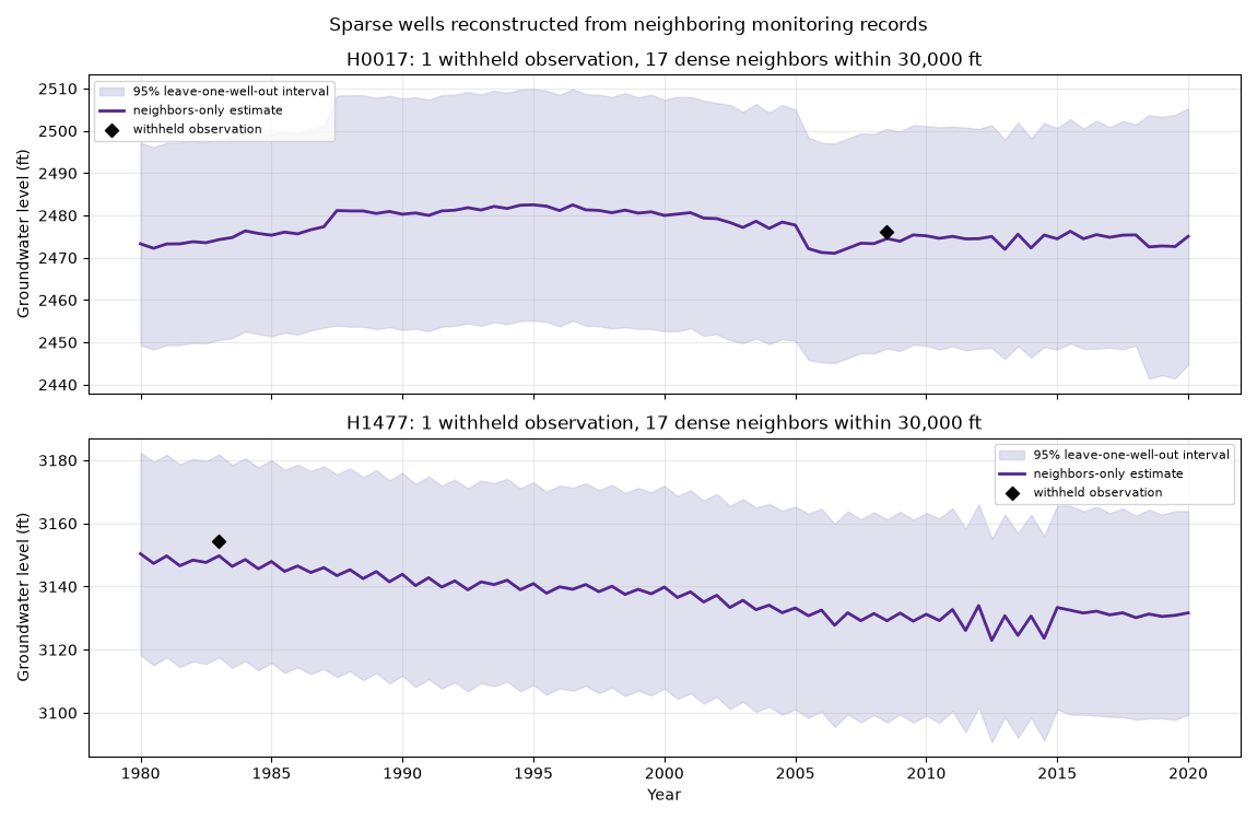
H0017: leave-one-well-out error=1.65 ft; dense neighbors within 30,000 ft=17
H1477: leave-one-well-out error=4.64 ft; dense neighbors within 30,000 ft=17

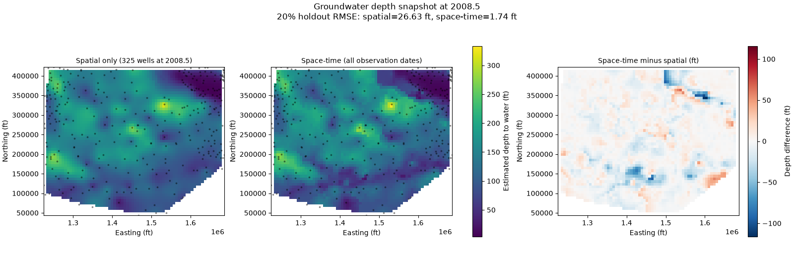
Grid snapshot at 2008.5

A snapshot at 2008.5 is a useful space-time demonstration because it has 325 contemporaneous observations: enough for a defensible spatial map, but fewer than the roughly 600 wells observed within two years of the snapshot. It is also a half-year date, so the fitted annual covariance is active.

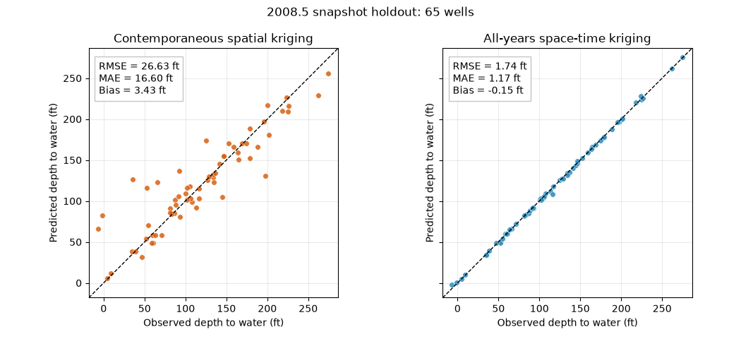
First withhold a reproducible 20% of the 2008.5 observations. The spatial baseline may use only the remaining observations from 2008.5. The space-time model also removes those exact rows, but retains measurements from other dates at the withheld wells. This tests whether temporal records improve prediction at a sparsely sampled snapshot; it is not a leave-one-well-out test.

Because 2008.5 is a half-year date, the space-time model is run twice — with and without the annual product term, at equal total temporal sill — so the holdout error isolates what the multiplicative quasi-periodic structure adds beyond a smooth long-term trend.

SNAPSHOT_TIME = 2008.5
HOLDOUT_FRACTION = 0.20
MAP_NX, MAP_NY = 70, 55

snapshot = data.loc[data["timeindex"] == SNAPSHOT_TIME].copy()
rng = np.random.default_rng(2026)
holdout_index = rng.choice(
    snapshot.index,
    size=int(np.ceil(HOLDOUT_FRACTION * len(snapshot))),
    replace=False,
)
snapshot_train = snapshot.drop(index=holdout_index)
snapshot_holdout = snapshot.loc[holdout_index]
spacetime_train = data.drop(index=holdout_index)


def krige_spatial_depth(train, grid_coord):
    """Ordinary kriging of depth to water from one time slice."""
    model = Kriging(ndim=2, nvar=1, neglect_error=False, verbose=0)
    model.set_obs(
        ivar=1,
        coord=train[["x", "y"]].to_numpy(),
        value=train["depth_to_water"].to_numpy(),
        variance=np.full(len(train), OBS_VARIANCE),
    )
    model.set_vgm(
        ivar=1,
        jvar=1,
        vtype=spatial_spec["vtype"],
        nugget=spatial_spec["nugget"],
        sill=spatial_spec["sill"],
        a_major=spatial_spec["a_major"],
        a_minor1=spatial_spec["a_major"],
        a_minor2=spatial_spec["a_major"],
    )
    model.set_grid(coord=grid_coord)
    model.set_search(ivar=1, nmax=NMAX, maxdist=MAXDIST)
    model.solve()
    result = model.get_results()
    del model
    return result


def krige_spacetime_depth(train, grid_coord, grid_time, temporal_model=temporal):
    """Space-time kriging of depth to water at one or more grid times.

    ``temporal_model`` selects the temporal marginal — the full Gaussian +
    annual product by default, or ``temporal_background`` to drop the annual
    term while keeping the same total sill and range.
    """
    model = SpaceTimeKriging(nvar=1, neglect_error=False, verbose=False)
    model.set_st_model("sum_metric", transform="linear", at=decay_range)
    model.set_obs(
        ivar=1,
        coord=np.column_stack([
            train["x"].to_numpy(),
            train["y"].to_numpy(),
            np.zeros(len(train)),
        ]),
        value=train["depth_to_water"].to_numpy(),
        time=train["timeindex"].to_numpy(),
        variance=np.full(len(train), OBS_VARIANCE),
    )
    model.set_vgm(
        ivar=1,
        jvar=1,
        vtype=spatial_spec["vtype"],
        nugget=spatial_spec["nugget"],
        sill=spatial_spec["sill"],
        a_major=spatial_spec["a_major"],
        a_minor1=spatial_spec["a_major"],
        a_minor2=spatial_spec["a_major"],
    )
    temporal_model.apply_temporal_to(model, ivar=1, jvar=1)
    model.set_vgm_joint_sills(1, 1, 0.0)
    model.set_grid(
        coord=np.column_stack([grid_coord, np.zeros(len(grid_coord))]),
        time=np.broadcast_to(grid_time, len(grid_coord)),
    )
    model.set_search(
        ivar=1,
        time_at=spatial_spec["a_major"] / decay_range,
        nmax=NMAX, maxdist=MAXDIST
    )
    model.solve()
    result = model.get_results(copy=True)
    del model
    return result


# Predict the withheld 2008.5 observations with both workflows.
holdout_coord = snapshot_holdout[["x", "y"]].to_numpy()
spatial_cv, spatial_cv_var = krige_spatial_depth(
    snapshot_train,
    holdout_coord,
)
spacetime_cv, spacetime_cv_var = krige_spacetime_depth(
    spacetime_train,
    holdout_coord,
    SNAPSHOT_TIME,
)
# Same space-time model but with the annual product term removed (equal total
# sill) — isolates what the multiplicative quasi-periodic structure contributes.
spacetime_noannual_cv, _ = krige_spacetime_depth(
    spacetime_train,
    holdout_coord,
    SNAPSHOT_TIME,
    temporal_model=temporal_background,
)
holdout_true = snapshot_holdout["depth_to_water"].to_numpy()


def validation_metrics(estimate):
    """Return RMSE, MAE, and bias against the snapshot holdout."""
    residual = np.asarray(estimate) - holdout_true
    return {
        "rmse": float(np.sqrt(np.mean(residual ** 2))),
        "mae": float(np.mean(np.abs(residual))),
        "bias": float(np.mean(residual)),
    }


spatial_metrics = validation_metrics(spatial_cv)
spacetime_metrics = validation_metrics(spacetime_cv)
spacetime_noannual_metrics = validation_metrics(spacetime_noannual_cv)
print(
    f"{SNAPSHOT_TIME:.1f} holdout ({len(snapshot_holdout)}/{len(snapshot)} wells): "
    f"spatial RMSE={spatial_metrics['rmse']:.2f} ft, "
    f"space-time (no annual) RMSE={spacetime_noannual_metrics['rmse']:.2f} ft, "
    f"space-time (+annual product) RMSE={spacetime_metrics['rmse']:.2f} ft"
)

2008.5 holdout (65/325 wells): spatial RMSE=26.63 ft, space-time (no annual) RMSE=1.89 ft, space-time (+annual product) RMSE=1.74 ft

Compare holdout predictions

The same withheld observations are compared against both models. Points on the dashed 1:1 line are predicted exactly. Shared square axes make departures from that line directly comparable between panels.

value_min = min(
    holdout_true.min(),
    np.min(spatial_cv),
    np.min(spacetime_cv),
)
value_max = max(
    holdout_true.max(),
    np.max(spatial_cv),
    np.max(spacetime_cv),
)
padding = 0.04 * (value_max - value_min)
plot_limits = (value_min - padding, value_max + padding)

fig, axes = plt.subplots(1, 2, figsize=(10.5, 4.8), sharex=True, sharey=True)
for ax, estimate, metrics, title, color in [
    (
        axes[0],
        spatial_cv,
        spatial_metrics,
        "Contemporaneous spatial kriging",
        "#d95f0e",
    ),
    (
        axes[1],
        spacetime_cv,
        spacetime_metrics,
        "All-years space-time kriging",
        "#2b8cbe",
    ),
]:
    ax.scatter(
        holdout_true,
        estimate,
        s=30,
        color=color,
        edgecolor="white",
        linewidth=0.45,
        alpha=0.85,
    )
    ax.plot(plot_limits, plot_limits, color="black", ls="--", lw=1.0)
    ax.set(
        xlim=plot_limits,
        ylim=plot_limits,
        aspect="equal",
        xlabel="Observed depth to water (ft)",
        ylabel="Predicted depth to water (ft)",
        title=title,
    )
    ax.text(
        0.04,
        0.95,
        f"RMSE = {metrics['rmse']:.2f} ft\n"
        f"MAE = {metrics['mae']:.2f} ft\n"
        f"Bias = {metrics['bias']:.2f} ft",
        transform=ax.transAxes,
        va="top",
        bbox={"facecolor": "white", "edgecolor": "0.75", "alpha": 0.9},
    )
    ax.grid(alpha=0.25)

fig.suptitle(
    f"{SNAPSHOT_TIME:.1f} snapshot holdout: {len(snapshot_holdout)} wells",
    fontsize=12,
)
fig.tight_layout()
plt.show()

Map contemporaneous-only and space-time estimates

Refit both maps with all 2008.5 observations restored. Cells outside the snapshot monitoring network’s convex hull are masked to avoid presenting unsupported extrapolation. The difference panel shows where observations from other dates change the 2008.5 estimate.

gx, gy = np.meshgrid(
    np.linspace(snapshot["x"].min(), snapshot["x"].max(), MAP_NX),
    np.linspace(snapshot["y"].min(), snapshot["y"].max(), MAP_NY),
)
map_coord = np.column_stack([gx.ravel(), gy.ravel()])
inside = Delaunay(snapshot[["x", "y"]].to_numpy()).find_simplex(map_coord) >= 0

spatial_map_inside, _ = krige_spatial_depth(snapshot, map_coord[inside])
spacetime_map_inside, _ = krige_spacetime_depth(
    data,
    map_coord[inside],
    SNAPSHOT_TIME,
)

spatial_map = np.full(len(map_coord), np.nan)
spacetime_map = np.full(len(map_coord), np.nan)
spatial_map[inside] = spatial_map_inside
spacetime_map[inside] = spacetime_map_inside
spatial_map = spatial_map.reshape(MAP_NY, MAP_NX)
spacetime_map = spacetime_map.reshape(MAP_NY, MAP_NX)
difference_map = spacetime_map - spatial_map

depth_min = np.nanmin([spatial_map, spacetime_map])
depth_max = np.nanmax([spatial_map, spacetime_map])
diff_limit = np.nanmax(np.abs(difference_map))
extent = [gx.min(), gx.max(), gy.min(), gy.max()]

fig, axes = plt.subplots(1, 3, figsize=(16, 5.2), constrained_layout=True)
for ax, values, title in [
    (
        axes[0],
        spatial_map,
        f"Spatial only ({len(snapshot)} wells at {SNAPSHOT_TIME:.1f})",
    ),
    (
        axes[1],
        spacetime_map,
        "Space-time (all observation dates)",
    ),
]:
    image = ax.imshow(
        values,
        origin="lower",
        extent=extent,
        cmap="viridis",
        vmin=depth_min,
        vmax=depth_max,
        aspect="equal",
    )
    ax.scatter(
        snapshot["x"],
        snapshot["y"],
        s=3,
        color="black",
        alpha=0.35,
    )
    ax.set_title(title, fontsize=10)
    ax.set_xlabel("Easting (ft)")
    ax.set_ylabel("Northing (ft)")

fig.colorbar(
    image,
    ax=axes[:2],
    shrink=0.83,
    label="Estimated depth to water (ft)",
)

diff_image = axes[2].imshow(
    difference_map,
    origin="lower",
    extent=extent,
    cmap="RdBu_r",
    vmin=-diff_limit,
    vmax=diff_limit,
    aspect="equal",
)
axes[2].set_title("Space-time minus spatial (ft)", fontsize=10)
axes[2].set_xlabel("Easting (ft)")
axes[2].set_ylabel("Northing (ft)")
fig.colorbar(diff_image, ax=axes[2], shrink=0.83, label="Depth difference (ft)")
fig.suptitle(
    f"Groundwater depth snapshot at {SNAPSHOT_TIME:.1f}\n"
    f"20% holdout RMSE: spatial={spatial_metrics['rmse']:.2f} ft, "
    f"space-time={spacetime_metrics['rmse']:.2f} ft",
    fontsize=12,
)
plt.show()