Ordinary Kriging + SGSIM

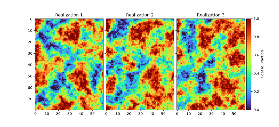
This example shows how to run SGSIM ordinary kriging and plot the interpolated field.

from krigekit import Kriging
import pandas as pd
import matplotlib.pyplot as plt
from mpl_toolkits.axes_grid1 import ImageGrid

data = pd.read_csv("../../test_data/pc2d.csv")
grid = pd.read_csv("../../test_data/grid2d.csv")

# nsim is the number of realizations
k = Kriging(nsim=3, bounds=[0,1])
k.set_obs(ivar=1, coord=data[["x", "y"]], value=data["pc"])
k.set_grid(coord=grid[["x", "y"]])
k.set_vgm(ivar=1, jvar=1, vtype="sph", sill=0.12, a_major=5000.0)
k.set_sim()
k.set_search(nmax=100)
k.solve()
df = k.get_result_df()
del k
print(df)

fig = plt.figure(figsize=(11, 5))
axs = ImageGrid(fig, 111,  # similar to subplot(111)
                nrows_ncols=(1, 3),
                axes_pad=0.1,
                label_mode="L",
                cbar_mode="single", cbar_size="7%", cbar_pad="2%"
                )

for i, ax in enumerate(axs):
    est = df[f"sim_{i+1}"].values.reshape([80, 60])
    im = ax.imshow(est, cmap="turbo", vmin=0, vmax=1)
    ax.set(title=f"Realization {i+1}")
ax.cax.colorbar(im, label="Coarse Fraction")

             x          y     sim_1     sim_2     sim_3  variance
0     573349.0  4400382.0  1.000000  1.000000  0.934483  0.014143
1     573554.0  4400525.0  1.000000  1.000000  1.000000  0.014277
2     573759.0  4400669.0  1.000000  1.000000  0.810030  0.025546
3     573964.0  4400812.0  1.000000  1.000000  0.769205  0.007997
4     574169.0  4400956.0  0.856978  0.898717  0.735295  0.009388
...        ...        ...       ...       ...       ...       ...
4795  595941.0  4392091.0  0.405936  0.525427  0.777810  0.007974
4796  596146.0  4392234.0  0.419499  0.518474  0.910027  0.011890
4797  596351.0  4392377.0  0.405917  0.550114  0.758689  0.007830
4798  596555.0  4392521.0  0.431009  0.553035  0.878958  0.008465
4799  596760.0  4392664.0  0.354609  0.525965  0.940438  0.019647

[4800 rows x 6 columns]

<matplotlib.colorbar.Colorbar object at 0x7d2987d9a610>

Change Seed

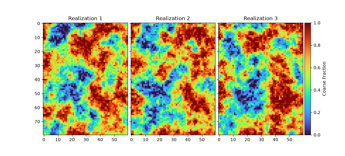
Let’s change seed number and see how different the results are.

k = Kriging(nsim=3, bounds=[0,1], seed=1000)
k.set_obs(ivar=1, coord=data[["x", "y"]], value=data["pc"])
k.set_grid(coord=grid[["x", "y"]])
k.set_vgm(ivar=1, jvar=1, vtype="sph", sill=0.12, a_major=5000.0)
k.set_sim()
k.set_search(nmax=100)
k.solve()
df = k.get_result_df()
del k
print(df)

fig = plt.figure(figsize=(11, 5))
axs = ImageGrid(fig, 111,  # similar to subplot(111)
                nrows_ncols=(1, 3),
                axes_pad=0.1,
                label_mode="L",
                cbar_mode="single", cbar_size="7%", cbar_pad="2%"
                )

for i, ax in enumerate(axs):
    est = df[f"sim_{i+1}"].values.reshape([80, 60])
    im = ax.imshow(est, cmap="turbo", vmin=0, vmax=1)
    ax.set(title=f"Realization {i+1}")
ax.cax.colorbar(im, label="Coarse Fraction")

             x          y     sim_1     sim_2     sim_3  variance
0     573349.0  4400382.0  0.930852  0.995609  0.750976  0.013098
1     573554.0  4400525.0  0.974483  1.000000  0.805975  0.018788
2     573759.0  4400669.0  0.849792  0.837587  0.843582  0.008706
3     573964.0  4400812.0  0.827087  0.968541  1.000000  0.013434
4     574169.0  4400956.0  1.000000  0.919989  1.000000  0.008672
...        ...        ...       ...       ...       ...       ...
4795  595941.0  4392091.0  0.556118  0.867091  0.423065  0.021341
4796  596146.0  4392234.0  0.442233  0.751838  0.704909  0.011170
4797  596351.0  4392377.0  0.519492  0.704493  0.797495  0.007828
4798  596555.0  4392521.0  0.629894  0.790397  0.935313  0.015007
4799  596760.0  4392664.0  0.560905  0.895621  0.962170  0.009910

[4800 rows x 6 columns]

<matplotlib.colorbar.Colorbar object at 0x7d298505b790>