Note
Go to the end to download the full example code.
Variogram fitting for space-time groundwater levels#
This example uses VariogramModel for the separate spatial
and temporal marginals, then composes them in
SpaceTimeVariogramModel to fit the joint sum-metric
coupling. The observations come from obs_gwlevel.csv.
The two marginals require different observation-pair definitions:
The spatial marginal uses one long-term mean depth-to-water value per well.
The temporal marginal uses pairs from the same well only. Pairing different wells would mix spatial differences into the temporal variogram.
Both fits follow the class workflow:
set_obs() -> calc_experimental() -> calc_average() -> set_vgm() -> fit().
The temporal model contains a slowly varying Gaussian background and a weaker annual covariance. The annual component is represented by a Gaussian structure multiplied by a hole-effect structure:
The hole-effect range is fixed numerically at 0.5 year because krigekit’s hole-effect covariance is \(\cos(\pi u/a)\), with period \(2a\). The two Gaussian ranges are fitted separately so the annual amplitude may decay at a different rate from the background covariance.
from pathlib import Path

import matplotlib.pyplot as plt
import numpy as np
import pandas as pd

from krigekit import SpaceTimeVariogramModel, VariogramModel


def _find_data_dir():
    """Locate ``test_data`` for direct and Sphinx-Gallery execution."""
    candidates = []
    if "__file__" in globals():
        candidates.append(Path(__file__).resolve().parents[2] / "test_data")
    cwd = Path.cwd().resolve()
    candidates.extend([
        cwd / "test_data",
        cwd.parent / "test_data",
        cwd.parent.parent / "test_data",
    ])
    for candidate in candidates:
        if candidate.exists():
            return candidate
    raise FileNotFoundError("Could not locate the test_data directory.")


def _calc_within_well_cloud(data, cutoff):
    """Calculate and combine temporal clouds without cross-well pairs."""
    clouds = []
    for _, group in data.groupby("WellID", sort=False):
        if len(group) < 2:
            continue
        well_model = VariogramModel()
        well_model.set_obs(
            group["timeindex"].to_numpy(dtype=float),
            group["depth_to_water"].to_numpy(dtype=float),
        )
        cloud = well_model.calc_experimental(
            cutoff=cutoff,
            verbose=False,
        )
        cloud = cloud.loc[cloud["distance"] > 0.0]
        if len(cloud):
            clouds.append(cloud)
    if not clouds:
        raise ValueError("no within-well temporal pairs were found")
    return pd.concat(clouds, ignore_index=True)


DATA_DIR = _find_data_dir()
SPATIAL_CUTOFF = 120_000.0
SPATIAL_WIDTH = 5_000.0
TEMPORAL_CUTOFF = 20.0
TEMPORAL_WIDTH = 0.5
MIN_WELL_OBS = 10
MIN_TEMPORAL_PAIRS = 30
JOINT_MAXOBS = 2_500
JOINT_MIN_PAIRS = 30

data = pd.read_csv(DATA_DIR / "obs_gwlevel.csv")
data["depth_to_water"] = data["dem10"] - data["sl_lev_va"]

print(
    f"{len(data):,} observations at {data['WellID'].nunique():,} wells, "
    f"{data['timeindex'].min():.1f}-{data['timeindex'].max():.1f}"
)
23,075 observations at 988 wells, 1978.0-2022.0
Fit the spatial marginal#
Long-term well means suppress temporal fluctuations and isolate the persistent spatial pattern. The count threshold avoids unstable means from short records.
well_mean = (
    data.groupby("WellID")
    .agg(
        x=("x", "first"),
        y=("y", "first"),
        depth=("depth_to_water", "mean"),
        count=("depth_to_water", "size"),
    )
    .query("count >= @MIN_WELL_OBS")
)

spatial = VariogramModel()
spatial.set_obs(
    well_mean[["x", "y"]].to_numpy(dtype=float),
    well_mean["depth"].to_numpy(dtype=float),
)
spatial.calc_experimental(cutoff=SPATIAL_CUTOFF, verbose=False)
spatial.calc_average(h_width=SPATIAL_WIDTH)
spatial.set_vgm(
    vtype="sph",
    nugget=50.0,
    sill=3_400.0,
    a_major=100_000.0,
)
spatial.fit(
    p0=(3_400.0, 100_000.0, 50.0),
    bounds=(
        (0.0, 1_000.0, 0.0),
        (10_000.0, 300_000.0, 1_000.0),
    ),
    weight_col=("variogram", "count"),
    inplace=True,
)
spatial.set_anisotropy(ratio_minor1=1.0, ratio_minor2=1.0)

spatial_spec = spatial.to_kriging_specs()[0]
print(
    "Spatial fit: "
    f"nugget={spatial_spec['nugget']:.1f}, "
    f"sill={spatial_spec['sill']:.1f}, "
    f"range={spatial_spec['a_major']:.0f} ft"
)
Spatial fit: nugget=0.0, sill=3518.8, range=102013 ft
Calculate the within-well temporal marginal#
Each temporary model receives one well’s time coordinate and measurements. Combining those clouds retains every admissible within-well pair while excluding all cross-well pairs.
temporal_cloud = _calc_within_well_cloud(data, TEMPORAL_CUTOFF)

temporal = VariogramModel()
temporal.raw_variogram_ = temporal_cloud
temporal_average = temporal.calc_average(h_width=TEMPORAL_WIDTH)
temporal_average = temporal_average.loc[
    temporal_average[("variogram", "count")] >= MIN_TEMPORAL_PAIRS
].copy()
temporal.avg_variogram_ = temporal_average

print(f"Within-well temporal pairs: {len(temporal_cloud):,}")
print(f"Occupied temporal bins: {len(temporal_average):,}")
Within-well temporal pairs: 442,911
Occupied temporal bins: 40
Fit the Gaussian and annual product structures#
set_vgm() defines the covariance groups before fitting:
an additive Gaussian background;
a Gaussian envelope for the seasonal covariance;
a hole-effect covariance multiplied into structure 2.
fit() normally estimates one sill and range per structure plus one
trailing nugget. The hole-effect sill and range are constrained to narrow
intervals around 1 and 0.5 year, respectively, fixing the annual period while
retaining the standard class fitting machinery.
The flat parameter order follows the order of the three set_vgm() calls:
background_sill, background_range,
seasonal_sill, seasonal_decay_range,
hole_effect_sill, hole_effect_range,
nugget
Thus the initial vector below means:
(35 ft², 30 yr, 2.5 ft², 30 yr, 1, 0.5 yr, 4 ft²)
The background and seasonal sills and ranges, plus the nugget, are fitted.
hole_effect_sill is fixed near 1 so it only modulates the seasonal
Gaussian covariance, and hole_effect_range is fixed near 0.5 year to
impose a one-year period.
temporal.set_vgm(
    vtype="gau",
    nugget=4.0,
    sill=35.0,
    a_major=30.0,
)
temporal.set_vgm(
    vtype="gau",
    sill=2.5,
    a_major=30.0,
)
temporal.set_vgm(
    vtype="hol",
    sill=1.0,
    a_major=0.5,
    product=True,
)

temporal.fit(
    # (background sill, background range,
    #  seasonal sill, seasonal decay range,
    #  hole-effect sill, hole-effect range, nugget)
    p0=(35.0, 30.0, 2.5, 30.0, 1.0, 0.5, 4.0),
    bounds=(
        # Lower bounds in the same order as p0.
        (0.0, 1.0, 0.0, 1.0, 1.0 - 1.0e-8, 0.5 - 1.0e-8, 0.0),
        # Upper bounds in the same order as p0.
        (100.0, 100.0, 20.0, 100.0, 1.0 + 1.0e-8, 0.5 + 1.0e-8, 50.0),
    ),
    weight_col=("variogram", "count"),
    inplace=True,
    maxfev=50_000,
)

temporal_specs = temporal.to_temporal_specs()
background_spec, seasonal_spec, annual_spec = temporal_specs
print(
    "Temporal fit: "
    f"nugget={background_spec['nugget']:.2f}, "
    f"background sill={background_spec['sill']:.2f}, "
    f"background range={background_spec['at_k']:.2f} yr, "
    f"seasonal sill={seasonal_spec['sill']:.2f}, "
    f"seasonal decay range={seasonal_spec['at_k']:.2f} yr, "
    f"annual period={2.0 * annual_spec['at_k']:.2f} yr"
)

print("Temporal SpaceTimeKriging specifications:")
for spec in temporal_specs:
    print(f"  {spec}")
Temporal fit: nugget=3.45, background sill=36.15, background range=32.86 yr, seasonal sill=2.41, seasonal decay range=44.02 yr, annual period=1.00 yr
Temporal SpaceTimeKriging specifications:
  {'vtype': 'gau', 'nugget': 3.4470114025181644, 'sill': 36.15465266717194, 'at_k': 32.85500578144071, 'product': False}
  {'vtype': 'gau', 'nugget': 0.0, 'sill': 2.409456061274512, 'at_k': 44.018630177206525, 'product': False}
  {'vtype': 'hol', 'nugget': 0.0, 'sill': 0.9999999997807563, 'at_k': 0.5000000046228206, 'product': True}
Fit the joint space-time coupling#
The boundary marginals alone do not determine how correlation behaves when both space and time lags are nonzero. A reproducible subset of observations is used to form the full two-dimensional lag surface without materializing all pair combinations from the 23,000-observation dataset.
The sum-metric model is
where \(q_S\) and \(q_T\) refine the amplitudes of the separately
fitted marginal shapes, \(b_{ST}\) is the coupling sill, and
\(f_T(u)\) is the linear temporal metric transform. With
time_sill=1, fitting at determines the conversion from years to the
dimensionless temporal part of the joint distance.
The flat fit vector is:
There is one joint_sill per spatial structure. This example has one
spherical spatial structure, so only one coupling sill is fitted.
joint = SpaceTimeVariogramModel(spatial=spatial, temporal=temporal)
joint.set_obs(
    data[["x", "y"]].to_numpy(dtype=float),
    data["depth_to_water"].to_numpy(dtype=float),
    times=data["timeindex"].to_numpy(dtype=float),
)
joint.calc_experimental(
    cutoff=SPATIAL_CUTOFF,
    t_cutoff=TEMPORAL_CUTOFF,
    maxobs=JOINT_MAXOBS,
    seed=2026,
    verbose=False,
)
joint_average = joint.calc_average(
    h_width=SPATIAL_WIDTH,
    t_col="time_lag",
    t_width=TEMPORAL_WIDTH,
)
joint_average = joint_average.loc[
    joint_average[("variogram", "count")] >= JOINT_MIN_PAIRS
].copy()
joint.avg_variogram_ = joint_average

joint.fit(
    model="sum_metric",
    transform="lin",
    time_sill=1.0,
    # (spatial scale, temporal scale, joint sill, at)
    p0=(1.0, 1.0, 100.0, 20.0),
    bounds=(
        (0.0, 0.0, 0.0, 1.0),
        (3.0, 5.0, 5_000.0, 100.0),
    ),
    weight_cap_quantile=0.90,
)

spatial_scale, temporal_scale, joint_sill, joint_at = (
    joint.sum_metric_params_
)
sum_metric_specs = joint.to_sum_metric_kriging_specs()

joint_hs = joint_average[("distance", "mean")].to_numpy()
joint_ht = joint_average[("time_lag", "mean")].to_numpy()
joint_gamma = joint_average[("variogram", "mean")].to_numpy()
joint_fitted = joint.calc_spacetime_sum_metric_variogram(joint_hs, joint_ht)
joint_no_coupling = (
    spatial_scale * spatial.variogram(joint_hs)
    + temporal_scale * temporal.variogram(joint_ht)
)
rmse_no_coupling = np.sqrt(np.mean((joint_no_coupling - joint_gamma) ** 2))
rmse_coupled = np.sqrt(np.mean((joint_fitted - joint_gamma) ** 2))

print(
    "Joint sum-metric fit: "
    f"spatial scale={spatial_scale:.3f}, "
    f"temporal scale={temporal_scale:.3f}, "
    f"joint sill={joint_sill:.2f} ft^2, "
    f"at={joint_at:.2f} yr"
)
print(
    f"Joint-surface RMSE: no coupling={rmse_no_coupling:.2f} ft^2, "
    f"with coupling={rmse_coupled:.2f} ft^2"
)
print("SpaceTimeKriging sum-metric setup:")
print(
    "  k.set_st_model("
    f"'sum_metric', transform='{sum_metric_specs['transform']}', "
    f"at={sum_metric_specs['at']:.3f}, "
    f"time_sill={sum_metric_specs['time_sill']:.1f})"
)
for index, spec in enumerate(sum_metric_specs["spatial_specs"], start=1):
    print(f"  # spatial structure {index}")
    print(f"  k.set_vgm(1, 1, **{spec})")
for index, spec in enumerate(sum_metric_specs["temporal_specs"], start=1):
    print(f"  # temporal structure {index}")
    print(f"  k.set_vgm_temporal(1, 1, **{spec})")
print(
    "  k.set_vgm_joint_sills("
    f"1, 1, {', '.join(f'{value:.6g}' for value in sum_metric_specs['joint_sills'])})"
)
print(f"  k.set_search(1, time_at={sum_metric_specs['time_at']:.3f})")
Joint sum-metric fit: spatial scale=0.894, temporal scale=0.332, joint sill=172.81 ft^2, at=23.70 yr
Joint-surface RMSE: no coupling=265.96 ft^2, with coupling=220.11 ft^2
SpaceTimeKriging sum-metric setup:
  k.set_st_model('sum_metric', transform='lin', at=23.696, time_sill=1.0)
  # spatial structure 1
  k.set_vgm(1, 1, **{'vtype': 'sph', 'nugget': 6.452606806738179e-14, 'sill': 3147.2725431905324, 'a_major': 102012.99882404084, 'a_minor1': 102012.99882404084, 'a_minor2': 102012.99882404084, 'azimuth': 0.0, 'dip': 0.0, 'plunge': 0.0, 'product': False})
  # temporal structure 1
  k.set_vgm_temporal(1, 1, **{'vtype': 'gau', 'nugget': 1.1428153663750509, 'sill': 11.986642284911639, 'at_k': 32.85500578144071, 'product': False})
  # temporal structure 2
  k.set_vgm_temporal(1, 1, **{'vtype': 'gau', 'nugget': 0.0, 'sill': 0.7988263135475683, 'at_k': 44.018630177206525, 'product': False})
  # temporal structure 3
  k.set_vgm_temporal(1, 1, **{'vtype': 'hol', 'nugget': 0.0, 'sill': 0.9999999997807563, 'at_k': 0.5000000046228206, 'product': True})
  k.set_vgm_joint_sills(1, 1, 172.815)
  k.set_search(1, time_at=23.696)
Plot both fitted marginals#
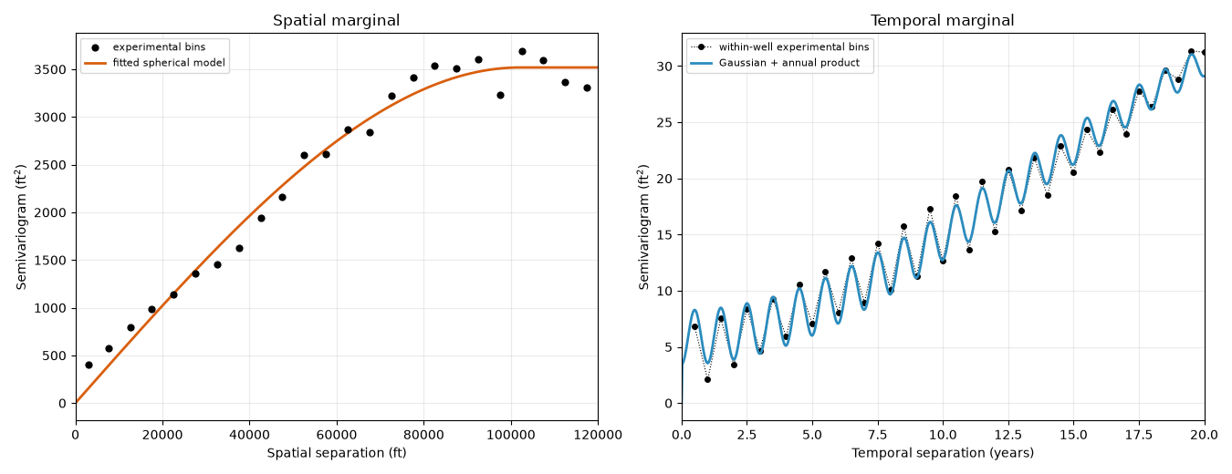
Integer temporal lags compare approximately the same season, while half-integer lags compare opposite seasons. The product covariance captures the resulting alternating semivariance.
fig, axes = plt.subplots(1, 2, figsize=(13.5, 5.2))

spatial_average = spatial.avg_variogram_
spatial_lag = np.linspace(0.0, SPATIAL_CUTOFF, 400)
axes[0].scatter(
    spatial_average[("distance", "mean")],
    spatial_average[("variogram", "mean")],
    s=24,
    color="black",
    label="experimental bins",
    zorder=3,
)
axes[0].plot(
    spatial_lag,
    spatial.variogram(spatial_lag),
    color="#d95f0e",
    lw=2.0,
    label="fitted spherical model",
)
axes[0].set(
    xlabel="Spatial separation (ft)",
    ylabel=r"Semivariogram (ft$^2$)",
    title="Spatial marginal",
    xlim=(0.0, SPATIAL_CUTOFF),
)

temporal_lag = np.linspace(0.0, TEMPORAL_CUTOFF, 800)
axes[1].plot(
    temporal_average[("distance", "mean")],
    temporal_average[("variogram", "mean")],
    color="black",
    marker="o",
    ms=4,
    lw=0.8,
    ls=":",
    label="within-well experimental bins",
)
axes[1].plot(
    temporal_lag,
    temporal.variogram(temporal_lag),
    color="#2b8cbe",
    lw=2.0,
    label="Gaussian + annual product",
)
axes[1].set(
    xlabel="Temporal separation (years)",
    ylabel=r"Semivariogram (ft$^2$)",
    title="Temporal marginal",
    xlim=(0.0, TEMPORAL_CUTOFF),
)

for ax in axes:
    ax.grid(alpha=0.25)
    ax.legend(fontsize=8)

fig.tight_layout()
plt.show()
Compare the full space-time lag surface#
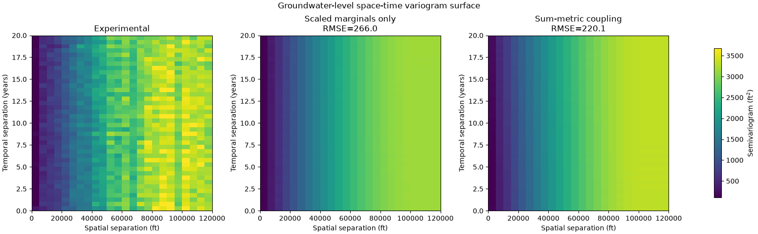
The coupling term improves the interior of the lag surface after the separately fitted marginal amplitudes are reconciled with the joint data.
joint_plot = pd.DataFrame({
    "hs_bin": (joint_hs / SPATIAL_WIDTH).astype(int),
    "ht_bin": (joint_ht / TEMPORAL_WIDTH).astype(int),
    "experimental": joint_gamma,
    "no_coupling": joint_no_coupling,
    "coupled": joint_fitted,
})
hs_bins = np.arange(int(SPATIAL_CUTOFF / SPATIAL_WIDTH))
ht_bins = np.arange(int(TEMPORAL_CUTOFF / TEMPORAL_WIDTH))


def _surface_grid(column):
    """Pivot one fitted/experimental column onto the common lag grid."""
    return (
        joint_plot.pivot_table(
            index="ht_bin",
            columns="hs_bin",
            values=column,
            aggfunc="mean",
        )
        .reindex(index=ht_bins, columns=hs_bins)
        .to_numpy()
    )


surface_values = [
    _surface_grid("experimental"),
    _surface_grid("no_coupling"),
    _surface_grid("coupled"),
]
vmin = np.nanquantile(surface_values[0], 0.02)
vmax = np.nanquantile(surface_values[0], 0.98)
extent = [0.0, SPATIAL_CUTOFF, 0.0, TEMPORAL_CUTOFF]

fig, axes = plt.subplots(1, 3, figsize=(15.5, 4.8), constrained_layout=True)
for ax, values, title in zip(
    axes,
    surface_values,
    [
        "Experimental",
        f"Scaled marginals only\nRMSE={rmse_no_coupling:.1f}",
        f"Sum-metric coupling\nRMSE={rmse_coupled:.1f}",
    ],
):
    image = ax.imshow(
        values,
        origin="lower",
        extent=extent,
        aspect="auto",
        cmap="viridis",
        vmin=vmin,
        vmax=vmax,
    )
    ax.set(
        xlabel="Spatial separation (ft)",
        ylabel="Temporal separation (years)",
        title=title,
    )

fig.colorbar(image, ax=axes, shrink=0.85, label=r"Semivariogram (ft$^2$)")
fig.suptitle("Groundwater-level space-time variogram surface")
plt.show()
Total running time of the script: (0 minutes 1.867 seconds)