Multi-Event Universal Kriging (MEUK) — synthetic replication

This example replicates the three-event synthetic application from Tonkin et al. (2016), Section 7.2, using krigekit’s co-kriging engine.

Problem setting. A 1-D aquifer transect (0–1000 m) contains one extraction well and one injection well. Three pumping/injection events are conducted at different flow rates and ambient gradient conditions. At each event, water levels are measured at a small number of monitoring locations. The goal is to estimate transmissivity \(T\) from all three datasets simultaneously.

Physical model. The water level at position \(x\) during event \(k\) is:

\[Z^{(k)}(x) = Z_0^{(k)} + \text{grad}^{(k)} \cdot x + \frac{1}{T}\,W^{(k)}(x) + \varepsilon^{(k)}(x)\]

where \(Z_0^{(k)}\) and \(\text{grad}^{(k)}\) are event-specific baseline head and ambient gradient, \(1/T\) is the shared hydraulic parameter, and \(W^{(k)}(x) = Q_k \ln(r_i / r_e)\) is the well influence function (log ratio of distances to injection and extraction wells). \(\varepsilon^{(k)}\) is a zero-mean spatially correlated residual.

MEUK vs UK. Standard Universal Kriging (UK) treats each event independently: it estimates \(Z_0^{(k)}\), \(\text{grad}^{(k)}\), and \(1/T_k\) from event \(k\) alone. Because \(1/T\) is physically shared, those per-event estimates are noisy and biased. MEUK (Multi-Event UK) sets up a single co-kriging system across all events with an augmented drift matrix that pools the \(1/T\) column while keeping per-event local drift columns separate. The pooled GLS estimate of \(1/T\) is statistically more efficient.

krigekit implementation. MEUK is expressed as co-kriging with:

• nvar = M — one variable per sampling event.

• unbias = 0 — user-supplied drift is the complete trend (no intercept added automatically).

• ndrift = Q_LOC * M + 1 — two local columns per event (\(1, x\)) plus one shared global column (\(W^{(k)}(x)\)).

• Zero cross-variograms between events (residuals are independent across events by assumption).

• nmax = N_TOT — each event’s kriging system may draw neighbours from all events, enabling the shared \(1/T\) column to pool information.

import numpy as np
import matplotlib.pyplot as plt
from krigekit import Kriging

# ---------------------------------------------------------------------------
# Constants
# ---------------------------------------------------------------------------
rng = np.random.default_rng(0)
escale   = 1e2           # overall noise scale
sigma    = 0.001*escale  # observation noise std dev
T_TRUE   = 300.0         # true transmissivity (m²/s)
X_WELL_E = 250.0         # extraction well position (m)
X_WELL_I = 750.0         # injection well position  (m)
R_MIN    = 5.0           # minimum radius to avoid log singularity

EVENTS = [
    dict(label='Event 1', n=23, grad= 0.0010, Q=10.0, Z0=50.0),
    dict(label='Event 2', n=18, grad=-0.0007, Q= 3.0, Z0=52.0),
    dict(label='Event 3', n=19, grad= 0.0005, Q=15.0, Z0=48.0),
]
M = len(EVENTS)

True water-level model

The analytical solution for steady-state head in a 1-D transect with one extraction well at \(x_e\) and one injection well at \(x_i\) is:

\[W^{(k)}(x) = Q_k \ln\!\left(\frac{r_i(x)}{r_e(x)}\right), \quad r_e = |x - x_e|,\; r_i = |x - x_i|\]

The coefficient \(\\beta = 1/T\) is shared across all events because transmissivity is a property of the aquifer, not of the pumping schedule. A minimum radius R_MIN prevents the log singularity at the well face.

def well_drift_col(x: np.ndarray, Q: float) -> np.ndarray:
    """Well-influence function W(x) = Q * ln(r_i / r_e)."""
    re = np.maximum(np.abs(x - X_WELL_E), R_MIN)
    ri = np.maximum(np.abs(x - X_WELL_I), R_MIN)
    return Q * np.log(ri / re)


def true_water_level(x: np.ndarray, ev: dict) -> np.ndarray:
    return ev['Z0'] + ev['grad'] * x + (1.0 / T_TRUE) * well_drift_col(x, ev['Q'])

Sampling observations

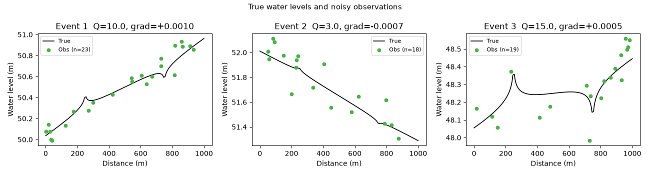
Monitoring locations are drawn uniformly along the transect for each event. Independent Gaussian noise with standard deviation \(\sigma\) is added to simulate measurement error and unresolved small-scale heterogeneity. The three events have different sample sizes (23, 18, 19), flow rates, and ambient gradients, reflecting realistic field conditions.

obs = []
for ev in EVENTS:
    x_k = np.sort(rng.uniform(0, 1000, ev['n']))
    z_k = true_water_level(x_k, ev) + rng.normal(0, sigma, ev['n'])
    obs.append(dict(x=x_k, z=z_k))

N_TOT = sum(ev['n'] for ev in EVENTS)

fig, axes = plt.subplots(1, M, figsize=(13, 3.5), sharey=False)
x_fine = np.linspace(0, 1000, 500)
for k, (ev, ax) in enumerate(zip(EVENTS, axes)):
    ax.plot(x_fine, true_water_level(x_fine, ev), 'k-', lw=1.2, label='True')
    ax.scatter(obs[k]['x'], obs[k]['z'], s=22, color='#4DAF4A',
               zorder=5, label=f"Obs (n={ev['n']})")
    ax.set_xlabel('Distance (m)')
    ax.set_ylabel('Water level (m)')
    ax.set_title(f"{ev['label']}  Q={ev['Q']}, grad={ev['grad']:+.4f}")
    ax.legend(fontsize=8)
fig.suptitle('True water levels and noisy observations', fontsize=11)
plt.tight_layout()
plt.show()

Variogram for residuals

After removing the true trend the residuals are \(\varepsilon(x) \sim \mathcal{N}(0, \sigma^2)\) by construction. We use a spherical model whose nugget and partial sill are each \(\sigma^2 / 2\), so the total sill equals \(\sigma^2\):

\[C(h) = \frac{\sigma^2}{2}\,\text{Sph}(h;\,a=80\,\text{m}) + \frac{\sigma^2}{2}\,\delta(h=0)\]

The same variogram is applied to every event (same aquifer, same measurement precision). Zero cross-variograms between events encode the assumption that residuals from different pumping tests are spatially independent.

VGM = dict(vtype='sph', nugget=5e-7*escale, sill=5e-7*escale, a_major=80.0)

Augmented drift design matrix

The MEUK drift matrix (Tonkin et al. 2016, Eq. 11) has ndrift = 7 columns arranged as a block structure:

[ V¹(x)  |    0    |    0    | W¹(x) ]   ← event 1 observation
[    0    | V²(x)  |    0    | W²(x) ]   ← event 2 observation
[    0    |    0    | V³(x)  | W³(x) ]   ← event 3 observation

where \(V^{(k)}(x) = [1,\, x]\) is the 2-column local drift for event \(k\) (intercept + spatial gradient) and \(W^{(k)}(x)\) is the well influence column shared across all events.

Each row corresponds to one observation. The block structure means that only the local drift columns belonging to the current event are non-zero, preventing the local parameters from bleeding across events. The last column is always populated and connects every observation to the shared transmissivity coefficient.

Q_LOC  = 2              # local drift cols per event: [1, x]
R_GLB  = 1              # global drift cols: [W^(k)(x)]
Q_TOT  = Q_LOC * M     # 6  (total local cols)
NDRIFT = Q_TOT + R_GLB # 7


def aug_obs_drift(k_idx: int, x: np.ndarray, Q: float) -> np.ndarray:
    """Return (n_k, NDRIFT) augmented drift matrix for event k (0-based)."""
    D = np.zeros((len(x), NDRIFT))
    D[:, k_idx * Q_LOC + 0] = 1.0                   # event-local intercept
    D[:, k_idx * Q_LOC + 1] = x                      # event-local gradient
    D[:, Q_TOT]              = well_drift_col(x, Q)  # shared well influence
    return D

MEUK via co-kriging

The three events are encoded as three variables (nvar=3). Setting unbias=0 tells krigekit that the user-supplied drift completely describes the trend — no automatic unbiasedness constraint is added on top.

Cross-variograms between events are set to zero (nugget and sill both 0), so the co-kriging weights assigned to other events’ observations are driven entirely by the shared drift column, not by any spatial cross-correlation.

km = Kriging(ndim=1, nvar=M, ndrift=NDRIFT, unbias=0)

for k, ev in enumerate(EVENTS):
    km.set_vgm(ivar=k+1, jvar=k+1,
               vtype=VGM['vtype'],
               nugget=VGM['nugget'], sill=VGM['sill'],
               a_major=VGM['a_major'])

for i in range(1, M + 1):
    for j in range(1, M + 1):
        if i != j:
            km.set_vgm(ivar=i, jvar=j, vtype='nug', nugget=0.0, sill=0.0, a_major=1.0)

for k, ev in enumerate(EVENTS):
    km.set_obs(ivar=k+1,
               coord=obs[k]['x'][:, None],
               value=obs[k]['z'])
    km.set_obs_drift(ivar=k+1,
                     drift=aug_obs_drift(k, obs[k]['x'], ev['Q']))

X_GRID = np.linspace(5.0, 995.0, 200)
km.set_grid(coord=X_GRID[:, None])

for k, ev in enumerate(EVENTS):
    km.set_grid_drift(drift=aug_obs_drift(k, X_GRID, ev['Q']), ivar=k+1)

for ivar in range(1, M + 1):
    km.set_search(ivar=ivar)

km.solve()

# get_results() → est (ngrid, M),  var (ngrid, M, M)
est_all, var_all = km.get_results()
meuk_est = [est_all[:, k] for k in range(M)]
meuk_var = [var_all[:, k, k] for k in range(M)]

UK per event (baseline)

For comparison, each event is kriged independently with its own full 3-column drift \([1,\, x,\, W^{(k)}(x)]\). This is the standard Universal Kriging approach: it fits \(1/T_k\) separately for each event, ignoring the constraint that transmissivity is a single shared physical parameter. With few observations per event the per-event \(1/T_k\) estimates are noisy.

uk_est, uk_var = [], []
for k, ev in enumerate(EVENTS):
    ob = obs[k]
    ku = Kriging(ndim=1, nvar=1, ndrift=Q_LOC + R_GLB, unbias=0)
    ku.set_vgm(ivar=1, jvar=1,
               vtype=VGM['vtype'],
               nugget=VGM['nugget'], sill=VGM['sill'],
               a_major=VGM['a_major'])
    ku.set_obs(ivar=1, coord=ob['x'][:, None], value=ob['z'])
    D_obs = np.column_stack([np.ones(ev['n']), ob['x'],
                             well_drift_col(ob['x'], ev['Q'])])
    ku.set_obs_drift(ivar=1, drift=D_obs)
    ku.set_grid(coord=X_GRID[:, None])
    D_grd = np.column_stack([np.ones(len(X_GRID)), X_GRID,
                             well_drift_col(X_GRID, ev['Q'])])
    ku.set_grid_drift(drift=D_grd)
    ku.set_search(ivar=1)
    ku.solve()
    z_hat, s2 = ku.get_results()
    uk_est.append(z_hat)
    uk_var.append(s2)

GLS trend coefficient comparison

The GLS (Generalised Least Squares) estimator of the drift coefficients \(\boldsymbol{\beta}\) minimises the weighted residual sum:

\[\hat{\boldsymbol{\beta}} = \left(\mathbf{F}^\top \mathbf{C}^{-1} \mathbf{F}\right)^{-1} \mathbf{F}^\top \mathbf{C}^{-1} \mathbf{z}\]

For UK, \(\mathbf{F}\) and \(\mathbf{C}\) are assembled per event independently. For MEUK, the normal equations are accumulated across all events before solving, so the shared \(1/T\) column pools information from all 60 observations. The pooled GLS estimate of \(1/T\) should be closer to the true value \(1/300 \approx 0.00333\).

def build_C(x: np.ndarray) -> np.ndarray:
    """Spherical covariance matrix C(h) for observations at positions x."""
    h = np.abs(x[:, None] - x[None, :]) / VGM['a_major']
    C = VGM['sill'] * np.where(h < 1, 1.0 - 1.5*h + 0.5*h**3, 0.0)
    np.fill_diagonal(C, VGM['nugget'] + VGM['sill'])
    return C


# UK: one GLS system per event
uk_beta = []
for k, (ev, ob) in enumerate(zip(EVENTS, obs)):
    C_k  = build_C(ob['x'])
    F_k  = np.column_stack([np.ones(ev['n']), ob['x'],
                            well_drift_col(ob['x'], ev['Q'])])
    Ci   = np.linalg.solve(C_k, np.eye(ev['n']))
    beta = np.linalg.solve(F_k.T @ Ci @ F_k, F_k.T @ Ci @ ob['z'])
    uk_beta.append(beta)

# MEUK: accumulate normal equations across all events, then solve once
A_full = np.zeros((NDRIFT, NDRIFT))
b_full = np.zeros(NDRIFT)
for k, (ev, ob) in enumerate(zip(EVENTS, obs)):
    C_k = build_C(ob['x'])
    F_k = aug_obs_drift(k, ob['x'], ev['Q'])
    Ci  = np.linalg.solve(C_k, np.eye(ev['n']))
    A_full += F_k.T @ Ci @ F_k
    b_full += F_k.T @ Ci @ ob['z']
meuk_beta = np.linalg.solve(A_full, b_full)

print(f"\n{'='*62}")
print(f"{'GLS trend coefficient comparison':^62}")
print(f"{'='*62}")
print(f"{'Parameter':<22} {'True':>9} {'MEUK':>9} {'UK-E1':>9} {'UK-E2':>9} {'UK-E3':>9}")
print(f"{'-'*62}")
print(f"{'1/T':22} {1/T_TRUE:9.5f} {meuk_beta[Q_TOT]:9.5f}"
      f" {uk_beta[0][2]:9.5f} {uk_beta[1][2]:9.5f} {uk_beta[2][2]:9.5f}")
for k, ev in enumerate(EVENTS):
    print(f"{'Z0 '+ev['label']:<22} {ev['Z0']:9.4f} {meuk_beta[k*Q_LOC]:9.4f}"
          f" {uk_beta[k][0]:9.4f}")
    print(f"{'grad '+ev['label']:<22} {ev['grad']:9.5f} {meuk_beta[k*Q_LOC+1]:9.5f}"
          f" {uk_beta[k][1]:9.5f}")
print(f"{'='*62}\n")

for k, ev in enumerate(EVENTS):
    z_true_g  = true_water_level(X_GRID, ev)
    rmse_uk   = np.sqrt(np.mean((uk_est[k]   - z_true_g)**2))
    rmse_meuk = np.sqrt(np.mean((meuk_est[k] - z_true_g)**2))
    print(f"{ev['label']}: RMSE  UK={rmse_uk:.5f}   MEUK={rmse_meuk:.5f}")

==============================================================
               GLS trend coefficient comparison
==============================================================
Parameter                   True      MEUK     UK-E1     UK-E2     UK-E3
--------------------------------------------------------------
1/T                      0.00333   0.00350   0.00036   0.00053   0.00489
Z0 Event 1               50.0000   49.9674   50.0377
grad Event 1             0.00100   0.00108   0.00093
Z0 Event 2               52.0000   52.0267   52.0526
grad Event 2            -0.00070  -0.00072  -0.00077
Z0 Event 3               48.0000   47.9768   47.9297
grad Event 3             0.00050   0.00054   0.00064
==============================================================

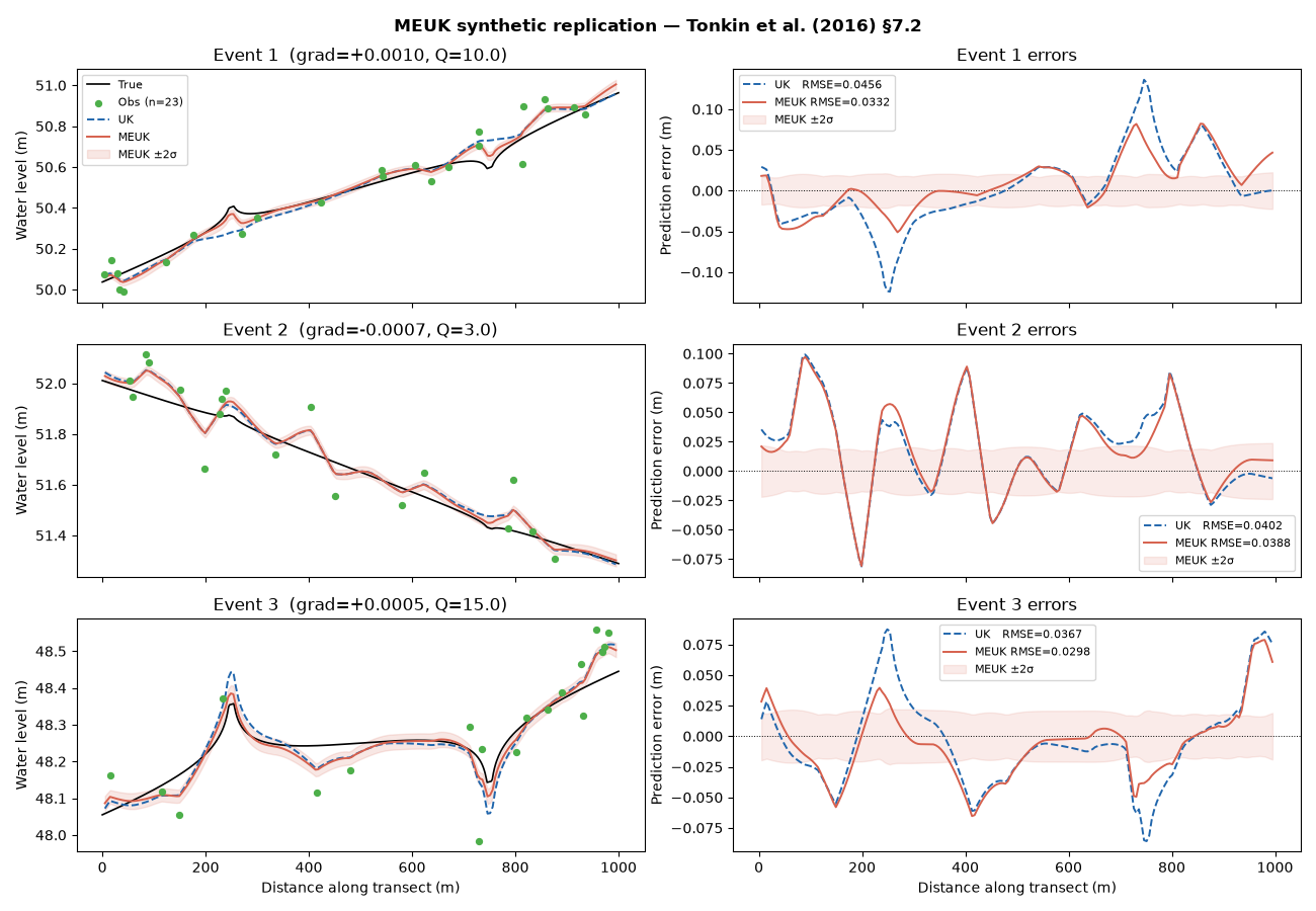
Event 1: RMSE  UK=0.04561   MEUK=0.03317
Event 2: RMSE  UK=0.04018   MEUK=0.03883
Event 3: RMSE  UK=0.03670   MEUK=0.02983

Prediction comparison — UK vs MEUK

Each row shows one pumping event. The left panel overlays the true water level (black), noisy observations (green), the independent UK estimate (blue dashed), and the MEUK estimate with its ±2σ uncertainty band (red).

The right panel shows the prediction error relative to the true water level. Because MEUK pools all events to estimate \(1/T\), it corrects the event-level bias in the trend fit and produces smaller errors, especially near the wells where the \(W^{(k)}(x)\) column dominates.

COLORS = {'uk': '#2166AC', 'meuk': '#D6604D', 'true': 'black', 'obs': '#4DAF4A'}

fig, axes = plt.subplots(M, 2, figsize=(13, 9), sharex=True)
fig.suptitle("MEUK synthetic replication — Tonkin et al. (2016) §7.2",
             fontsize=12, fontweight='bold')

for k, ev in enumerate(EVENTS):
    ax_p, ax_e = axes[k, 0], axes[k, 1]
    z_true_g = true_water_level(X_GRID, ev)
    z_fine   = true_water_level(x_fine, ev)
    err_uk   = uk_est[k]   - z_true_g
    err_meuk = meuk_est[k] - z_true_g
    sig_uk   = np.sqrt(np.maximum(uk_var[k],   0.0))
    sig_meuk = np.sqrt(np.maximum(meuk_var[k], 0.0))

    # Prediction panel
    ax_p.plot(x_fine, z_fine, '-', color=COLORS['true'], lw=1.2, label='True')
    ax_p.scatter(obs[k]['x'], obs[k]['z'], s=18, color=COLORS['obs'],
                 zorder=5, label=f"Obs (n={ev['n']})")
    ax_p.plot(X_GRID, uk_est[k],   '--', color=COLORS['uk'],   lw=1.4, label='UK')
    ax_p.plot(X_GRID, meuk_est[k], '-',  color=COLORS['meuk'], lw=1.4, label='MEUK')
    ax_p.fill_between(X_GRID,
                      meuk_est[k] - 2*sig_meuk,
                      meuk_est[k] + 2*sig_meuk,
                      color=COLORS['meuk'], alpha=0.15, label='MEUK ±2σ')
    ax_p.set_ylabel('Water level (m)')
    ax_p.set_title(f"{ev['label']}  (grad={ev['grad']:+.4f}, Q={ev['Q']})")
    if k == 0:
        ax_p.legend(fontsize=8, loc='upper left')

    # Error panel
    rmse_uk   = np.sqrt(np.mean(err_uk**2))
    rmse_meuk = np.sqrt(np.mean(err_meuk**2))
    ax_e.axhline(0, color='k', lw=0.7, ls=':')
    ax_e.plot(X_GRID, err_uk,   '--', color=COLORS['uk'],
              lw=1.4, label=f'UK   RMSE={rmse_uk:.4f}')
    ax_e.plot(X_GRID, err_meuk, '-',  color=COLORS['meuk'],
              lw=1.4, label=f'MEUK RMSE={rmse_meuk:.4f}')
    ax_e.fill_between(X_GRID, -2*sig_meuk, 2*sig_meuk,
                      color=COLORS['meuk'], alpha=0.12, label='MEUK ±2σ')
    ax_e.set_ylabel('Prediction error (m)')
    ax_e.set_title(f"{ev['label']} errors")
    ax_e.legend(fontsize=8)

for ax in axes[-1]:
    ax.set_xlabel('Distance along transect (m)')

plt.tight_layout()
plt.show()