Fitting a product-sum variogram for the CCl4 plume

This example isolates the variogram-fitting stage used by st_ok3d_ctet.py. The CCl4 dataset contains repeated measurements from 281 wells over about 13 years and a three-dimensional plume domain.

Concentrations are transformed to uniform quantile scores before fitting. This is intentional: QuantileTransformer defaults to output_distribution="uniform", whose theoretical variance is \(1/12\). The original kriging example historically called these values “normal scores”, although its plots and fitted sills were percentile-based.

The example demonstrates an important practical lesson: a five-parameter product-sum surface may have weakly identified temporal parameters when the experimental cloud contains few pairs close to both zero spatial lag and zero temporal lag. A constrained numerical optimum is a useful diagnostic, but it does not replace geological judgment or cross-validation.

from pathlib import Path

import matplotlib.pyplot as plt
import numpy as np
import pandas as pd
from sklearn.preprocessing import QuantileTransformer

from krigekit import SpaceTimeVariogramModel


def _find_data_dir():
    """Locate test_data when run directly or through Sphinx-Gallery."""
    candidates = []
    if "__file__" in globals():
        candidates.append(Path(__file__).resolve().parents[2] / "test_data")
    cwd = Path.cwd().resolve()
    candidates.extend([
        cwd / "test_data",
        cwd.parent / "test_data",
        cwd.parent.parent / "test_data",
    ])
    for candidate in candidates:
        if candidate.exists():
            return candidate
    raise FileNotFoundError("Could not locate the test_data directory.")


DATA_DIR = _find_data_dir()
MAX_HS = 5_500.0
MAX_HT = 13.0
HS_STEP = 500.0
HT_STEP = 0.5
MIN_PAIRS = 5
MIN_WELL_OBS = 7
Z_SCALE = 5.0

Load and transform the observations

Measurements duplicated at the same well, screen elevation, and decimal date are averaged. The fitted transformer is retained for inverse transformation in the kriging example.

data = pd.read_csv(DATA_DIR / "ctet.csv")
date = pd.to_datetime(data["time"], format="%m/%d/%Y %H:%M")
data["t"] = date.dt.year + date.dt.dayofyear / 365.0
data = (
    data.groupby(["well", "x", "y", "z", "t"], as_index=False)["CCl4"]
    .mean()
)

quantile_transform = QuantileTransformer(
    output_distribution="uniform",
    random_state=0,
)
data["uscore"] = quantile_transform.fit_transform(data[["CCl4"]]).ravel()

well_count = data.groupby("well").size()
selected_wells = well_count[well_count >= MIN_WELL_OBS].index
selected = data.loc[data["well"].isin(selected_wells)].reset_index(drop=True)

print(f"Observations after aggregation : {len(data):,}")
print(f"Wells                         : {data['well'].nunique()}")
print(f"Observations used for fitting : {len(selected):,}")
print(f"Uniform-score variance        : {data['uscore'].var(ddof=1):.5f}")
print(f"Theoretical uniform variance  : {1.0 / 12.0:.5f}")

Observations after aggregation : 3,823
Wells                         : 281
Observations used for fitting : 3,571
Uniform-score variance        : 0.08339
Theoretical uniform variance  : 0.08333

Calculate the experimental space-time variogram

The raw cloud retains physical XYZ distances. The anisotropic lag rotates and scales each lag vector using the same convention as the kriging engine. Here the vertical range is one fifth of the horizontal range.

coord = np.column_stack([
    selected["x"],
    selected["y"],
    selected["z"],
])
time = selected["t"].to_numpy()
score = selected["uscore"].to_numpy()

model = SpaceTimeVariogramModel()
model.set_obs(coord, score, times=time)
model.calc_experimental(
    cutoff=MAX_HS,
    t_cutoff=MAX_HT,
    anisotropy={"anis2": 1.0 / Z_SCALE},
    verbose=False,
)
average = model.calc_average(
    h_col="anisotropic_distance",
    h_width=HS_STEP,
    t_col="time_lag",
    t_width=HT_STEP,
)
average = average.loc[average[("variogram", "count")] >= MIN_PAIRS].copy()
model.avg_variogram_ = average

experimental = pd.DataFrame({
    "hs": average[("anisotropic_distance", "mean")].to_numpy(),
    "ht": average[("time_lag", "mean")].to_numpy(),
    "gamma": average[("variogram", "mean")].to_numpy(),
    "count": average[("variogram", "count")].to_numpy(),
})
experimental["hs_bin"] = (experimental["hs"] / HS_STEP).astype(int)
experimental["ht_bin"] = (experimental["ht"] / HT_STEP).astype(int)

print(f"Admissible observation pairs  : {len(model.raw_variogram_):,}")
print(f"Occupied fitting bins         : {len(experimental):,}")

Admissible observation pairs  : 6,320,157
Occupied fitting bins         : 286

Product-sum model and validity constraints

The fitted variogram is

\[\gamma(h_s,h_t) = a\,g_S(h_s) + b\,g_T(h_t) + p\,g_S(h_s)g_T(h_t),\]

where \(g_S\) is spherical and \(g_T\) is Gaussian, each normalized to unit sill. Conversion to krigekit’s covariance form requires

\[C_S(0)=a+p>0,\qquad C_T(0)=b+p>0,\qquad p\leq0.\]

These marginal-sill constraints are stronger and more useful than checking only \(a+b+p>0\).

hs = experimental["hs"].to_numpy()
ht = experimental["ht"].to_numpy()
gamma = experimental["gamma"].to_numpy()
count = experimental["count"].to_numpy()

# Cap pair-count weights so a few very populous short-lag bins do not dominate
# every other part of the surface.
bounds = [
    (0.0, 0.30),       # a
    (0.0, 0.20),       # b
    (-0.20, 0.0),      # p
    (1_000.0, 8_000.0),
    (1.0, MAX_HT),
]
# Multiple starting points reveal whether the objective has competing local
# minima.  The result with the smallest weighted objective is retained.
starts = [
    (0.10, 0.06, -0.005, 5_000.0, 9.0),
    (0.12, 0.04, -0.020, 3_000.0, 10.0),
    (0.10, 0.10, -0.010, 5_000.0, 5.0),
]
model.fit(
    model="product_sum",
    spatial_vtype="sph",
    temporal_vtype="gau",
    starts=starts,
    bounds=bounds,
    weight_cap_quantile=0.90,
)
automatic = model.spacetime_fit_result_
fits = model.spacetime_fit_results_
automatic_params = model.spacetime_params_.copy()

Inspect the automatic fit

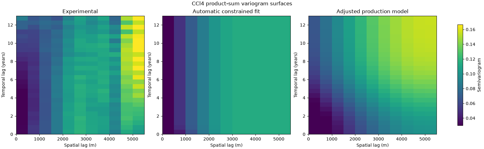
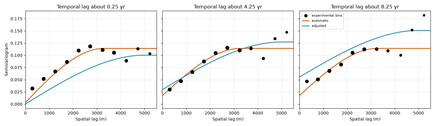
For this dataset the numerical optimum typically pushes the temporal marginal sill close to zero or a range to one of its bounds. That is a warning about identifiability, not evidence that the plume truly loses all temporal persistence at the fitted scale.

def print_params(label, params):
    """Print product-sum variogram and converted covariance parameters."""
    a, b, p, spatial_range, temporal_range = params
    sill_s = a + p
    sill_t = b + p
    k_ps = -p / (sill_s * sill_t)
    print(label)
    print(f"  a={a:.5f}, b={b:.5f}, p={p:.5f}")
    print(
        f"  spatial range={spatial_range:.1f} m, "
        f"temporal range={temporal_range:.2f} yr"
    )
    print(
        f"  covariance: sill_s={sill_s:.5f}, sill_t={sill_t:.5f}, "
        f"k_ps={k_ps:.4f}"
    )


print_params("Automatic constrained fit:", automatic_params)
for index, result in enumerate(fits, start=1):
    print(
        f"  start {index}: objective={result.fun:.6g}, "
        f"ranges=({result.x[3]:.0f} m, {result.x[4]:.2f} yr)"
    )

at_bounds = (
    np.isclose(automatic_params[3], bounds[3][0])
    or np.isclose(automatic_params[3], bounds[3][1])
    or np.isclose(automatic_params[4], bounds[4][0])
    or np.isclose(automatic_params[4], bounds[4][1])
)
weak_temporal_sill = automatic_params[1] + automatic_params[2] < 0.005
print(
    "Automatic-fit diagnostic: "
    f"range at bound={at_bounds}, weak temporal covariance sill={weak_temporal_sill}"
)

Automatic constrained fit:
  a=0.11398, b=0.01748, p=-0.01738
  spatial range=3276.5 m, temporal range=1.00 yr
  covariance: sill_s=0.09660, sill_t=0.00010, k_ps=1799.1083
  start 1: objective=0.00858786, ranges=(3276 m, 1.00 yr)
  start 2: objective=0.00916946, ranges=(3112 m, 10.32 yr)
  start 3: objective=0.00858786, ranges=(3276 m, 1.00 yr)
Automatic-fit diagnostic: range at bound=True, weak temporal covariance sill=True

Manually adjusted production model

The production model used by st_ok3d_ctet.py keeps a broader spatial range and a nine-year temporal range. These rounded values trade a modest increase in experimental-surface residual for interpretable plume continuity and better prediction behavior established during the original workflow.

This is not an invitation to tune by eye alone. In a production analysis, compare candidate models by blocked space-time cross-validation, including error and bias for the high-concentration tail after inverse transformation.

production_params = np.array([0.10, 0.06, -0.005, 5_000.0, 9.0])
print_params("Manually adjusted production model:", production_params)

automatic_rmse = np.sqrt(np.mean(
    (model.calc_spacetime_variogram(hs, ht, automatic_params) - gamma) ** 2
))
production_rmse = np.sqrt(np.mean(
    (model.calc_spacetime_variogram(hs, ht, production_params) - gamma) ** 2
))
print(f"Unweighted bin RMSE, automatic : {automatic_rmse:.5f}")
print(f"Unweighted bin RMSE, production: {production_rmse:.5f}")

Manually adjusted production model:
  a=0.10000, b=0.06000, p=-0.00500
  spatial range=5000.0 m, temporal range=9.00 yr
  covariance: sill_s=0.09500, sill_t=0.05500, k_ps=0.9569
Unweighted bin RMSE, automatic : 0.01846
Unweighted bin RMSE, production: 0.02397

Compare experimental and fitted surfaces

The numerical fit follows the most heavily supported bins more closely. The adjusted model deliberately preserves longer spatial and temporal continuity.

hs_grid = (np.arange(int(MAX_HS / HS_STEP)) + 0.5) * HS_STEP
ht_grid = (np.arange(int(MAX_HT / HT_STEP)) + 0.5) * HT_STEP
grid_hs, grid_ht = np.meshgrid(hs_grid, ht_grid)

experimental_grid = (
    experimental.pivot(index="ht_bin", columns="hs_bin", values="gamma")
    .reindex(index=np.arange(len(ht_grid)), columns=np.arange(len(hs_grid)))
    .to_numpy()
)
automatic_grid = model.calc_spacetime_variogram(
    grid_hs, grid_ht, automatic_params
)
production_grid = model.calc_spacetime_variogram(
    grid_hs, grid_ht, production_params
)

vmin = np.nanquantile(experimental_grid, 0.02)
vmax = np.nanquantile(experimental_grid, 0.98)
extent = [0.0, MAX_HS, 0.0, MAX_HT]

fig, axes = plt.subplots(1, 3, figsize=(15.5, 4.8), constrained_layout=True)
for ax, values, title in zip(
    axes,
    [experimental_grid, automatic_grid, production_grid],
    ["Experimental", "Automatic constrained fit", "Adjusted production model"],
):
    image = ax.imshow(
        values,
        origin="lower",
        extent=extent,
        aspect="auto",
        cmap="viridis",
        vmin=vmin,
        vmax=vmax,
    )
    ax.set(
        xlabel="Spatial lag (m)",
        ylabel="Temporal lag (years)",
        title=title,
    )

fig.colorbar(image, ax=axes, shrink=0.85, label="Semivariogram")
fig.suptitle("CCl4 product-sum variogram surfaces")
plt.show()

Compare representative spatial slices

Experimental bins nearest to three temporal lags are overlaid with both models. Slice plots make systematic range differences easier to see than a surface alone.

fig, axes = plt.subplots(1, 3, figsize=(14.5, 4.2), sharey=True)
for ax, target_ht in zip(axes, (0.25, 4.25, 8.25)):
    time_bin = int(target_ht / HT_STEP)
    section = experimental.loc[experimental["ht_bin"] == time_bin]
    line_hs = np.linspace(0.0, MAX_HS, 300)
    line_ht = np.full_like(line_hs, target_ht)
    ax.scatter(
        section["hs"],
        section["gamma"],
        s=np.clip(np.sqrt(section["count"]) / 2.0, 18.0, 70.0),
        color="black",
        label="experimental bins",
        zorder=3,
    )
    ax.plot(
        line_hs,
        model.calc_spacetime_variogram(line_hs, line_ht, automatic_params),
        color="#d95f0e",
        lw=2.0,
        label="automatic",
    )
    ax.plot(
        line_hs,
        model.calc_spacetime_variogram(line_hs, line_ht, production_params),
        color="#2b8cbe",
        lw=2.0,
        label="adjusted",
    )
    ax.set(
        xlabel="Spatial lag (m)",
        title=f"Temporal lag about {target_ht:.2f} yr",
        xlim=(0.0, MAX_HS),
    )
    ax.grid(alpha=0.25)

axes[0].set_ylabel("Semivariogram")
axes[-1].legend(fontsize=8)
fig.tight_layout()
plt.show()

Engine-ready production parameters

Convert the adjusted variogram coefficients to the covariance parameters expected by SpaceTimeKriging.

model.set_spacetime_params(production_params)
specs = model.to_spacetime_kriging_specs()
spatial_spec = specs["spatial_spec"]
temporal_spec = specs["temporal_spec"]

print("SpaceTimeKriging production setup:")
print(f"  k.set_st_model('product_sum', k_ps={specs['k_ps']:.6f})")
print(
    "  k.set_vgm(1, 1, vtype='sph', "
    f"sill={spatial_spec['sill']:.6f}, "
    f"a_major={spatial_spec['a_major']:.1f}, "
    f"a_minor1={spatial_spec['a_minor1']:.1f}, "
    f"a_minor2={spatial_spec['a_minor2']:.1f})"
)
print(
    "  k.set_vgm_temporal(1, 1, vtype='gau', "
    f"sill={temporal_spec['sill']:.6f}, "
    f"at_k={temporal_spec['at_k']:.2f})"
)
print(f"  k.set_search(1, time_at={specs['time_at']:.3f})")

SpaceTimeKriging production setup:
  k.set_st_model('product_sum', k_ps=0.956938)
  k.set_vgm(1, 1, vtype='sph', sill=0.095000, a_major=5000.0, a_minor1=5000.0, a_minor2=1000.0)
  k.set_vgm_temporal(1, 1, vtype='gau', sill=0.055000, at_k=9.00)
  k.set_search(1, time_at=959.596)