Fitting a 3-D anisotropic variogram

This example demonstrates the full 3-D anisotropic variogram workflow on a synthetic data set whose true model is known, so the fitted ranges can be checked against the ground truth.

The data are generated with unconditional sequential Gaussian simulation (SGSIM): a Gaussian random field is drawn on a regular 3-D grid directly from a known spherical model (no conditioning data), and a random subset of nodes is kept as the “samples”. We then:

• compute and cache the empirical variogram cloud (with 3-D lag angles),

• average it along the model’s fixed major / minor1 / minor2 axes with calc_directional_average(),

• fit sills and the three anisotropic ranges with fit_anisotropy().

Note

fit_anisotropy fits sills, ranges, and the nugget for a fixed orientation; the azimuth / dip / plunge angles are supplied, not fitted. Here (azimuth, dip, plunge) follow the engine convention and are exactly scipy’s extrinsic "zxy" Euler angles (dip positive down).

import matplotlib.pyplot as plt
import numpy as np

from krigekit import Kriging, VariogramModel
from krigekit.variogram import rotation_matrix_3d

Generate a 3-D field with unconditional SGSIM

The true model is a single anisotropic spherical structure. An unconditional simulation is set up by calling set_obs with empty observation arrays; the first visited node is then drawn from the prior N(0, sill) and later nodes condition only on previously simulated nodes.

TRUE = dict(
    vtype="sph", nugget=0.0, sill=1.0,
    a_major=30.0, a_minor1=12.0, a_minor2=8.0,
    azimuth=30.0, dip=20.0, plunge=0.0,
)

axis = np.arange(0.0, 90.0, 3.0)
gx, gy, gz = np.meshgrid(axis, axis, axis, indexing="ij")
grid = np.column_stack([gx.ravel(), gy.ravel(), gz.ravel()])

sim = Kriging(ndim=3, nvar=1, nsim=1, seed=2024)
sim.set_obs(ivar=1, coord=np.empty((0, 3)), value=np.empty((0,)))
sim.set_grid(coord=grid)
sim.set_vgm(ivar=1, jvar=1, **TRUE)
sim.set_sim()
sim.set_search(
    ivar=1,
    anis1=TRUE["a_minor1"] / TRUE["a_major"],
    anis2=TRUE["a_minor2"] / TRUE["a_major"],
    azimuth=TRUE["azimuth"], dip=TRUE["dip"],
    nmax=48
)
sim.solve()
field = np.asarray(sim.get_results()[0])

# Keep a random subset of nodes as irregular "samples" to estimate from.  The
# short minor2 range is data-hungry, so use enough samples to give the steep
# short-axis direction comparable pair support.
rng = np.random.default_rng(1)
sample_idx = rng.choice(len(grid), size=3000, replace=False)
sample_coord = grid[sample_idx]
sample_value = field[sample_idx]

print(f"Simulated field: {field.size} nodes, variance = {field.var():.3f} "
      f"(target sill {TRUE['sill']:.1f})")

Simulated field: 27000 nodes, variance = 1.026 (target sill 1.0)

Eyeball the anisotropy in 3-D

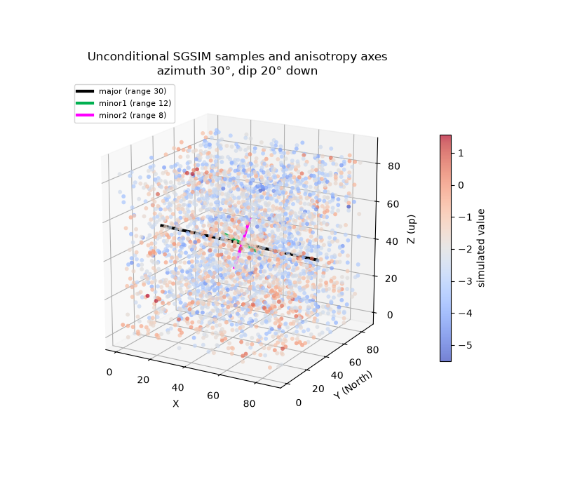
A 3-D scatter of the samples (coloured by value) shows the elongated high/low streaks of continuity. The three principal axes – scaled by their true ranges and drawn through the domain centre – let the azimuth and dip be read off directly: the long crimson (major) axis points along azimuth = 30 (clockwise from +Y/North) and dips 20 below horizontal.

# High-contrast axis colours so they stand out against the red/blue value map.
AXIS_COLORS = {"major": "black", "minor1": "#00b050", "minor2": "magenta"}
axis_names = ["major", "minor1", "minor2"]
# rotation_matrix_3d columns are (major, minor1, minor2) unit directions.
axis_dirs = rotation_matrix_3d(TRUE["azimuth"], TRUE["dip"], TRUE["plunge"]).T
axis_ranges = [TRUE["a_major"], TRUE["a_minor1"], TRUE["a_minor2"]]
center = grid.mean(axis=0)

fig = plt.figure(figsize=(8.0, 7.0))
ax3d = fig.add_subplot(111, projection="3d")
pts = ax3d.scatter(
    sample_coord[:, 0], sample_coord[:, 1], sample_coord[:, 2],
    c=sample_value, cmap="coolwarm", s=18, alpha=0.7, depthshade=False,
    edgecolors="none",
)
fig.colorbar(pts, ax=ax3d, shrink=0.6, pad=0.08, label="simulated value")

# Draw each principal axis as a double-headed line scaled by 1.6x its range so
# it stands out against the point cloud.
for name, vec, rng_ in zip(axis_names, axis_dirs, axis_ranges):
    end = 1.6 * rng_ * vec
    ax3d.plot(
        [center[0] - end[0], center[0] + end[0]],
        [center[1] - end[1], center[1] + end[1]],
        [center[2] - end[2], center[2] + end[2]],
        color=AXIS_COLORS[name], lw=3,
        label=f"{name} (range {rng_:.0f})",
    )

ax3d.set_xlabel("X")
ax3d.set_ylabel("Y (North)")
ax3d.set_zlabel("Z (up)")
ax3d.set_box_aspect((1, 1, 1))   # equal aspect so angles are not distorted
ax3d.view_init(elev=18, azim=-60)
ax3d.set_title(
    f"Unconditional SGSIM samples and anisotropy axes\n"
    f"azimuth {TRUE['azimuth']:.0f}°, dip {TRUE['dip']:.0f}° down"
)
ax3d.legend(loc="upper left", fontsize=8)
plt.show()

Empirical and directional variograms

The model orientation (azimuth/dip/plunge) is fixed up front; calc_directional_average then bins the cloud along the major, minor1, and minor2 axes. include_minor2=True (inferred automatically here) keeps the vertical axis so all three anisotropic ranges can be fitted.

model = VariogramModel()
model.set_obs(sample_coord, sample_value)
model.set_vgm(
    vtype="sph", nugget=0.0, sill=1.0,
    a_major=35.0, a_minor1=15.0, a_minor2=10.0,
    azimuth=TRUE["azimuth"], dip=TRUE["dip"], plunge=TRUE["plunge"],
)

model.calc_experimental(cutoff=36.0, calc_angle=True, verbose=False)
dir_avg = model.calc_directional_average(
    h_bins=18,
    cutoff=36.0,
    angle_tol=20.0,
)

# Pair counts can differ strongly by direction, especially for the steep,
# shortest minor2 axis.  Normalize count weights within each axis so the fit
# does not let the better-populated major/minor1 directions dominate minor2.
dir_avg["axis_weight"] = (
    dir_avg["count"] / dir_avg.groupby("axis", observed=True)["count"].transform("sum")
)

# The synthetic field has no nugget, so fit_nugget=False keeps the fit stable
# (fitting a spurious nugget would otherwise trade sill for nugget).
model.fit_anisotropy(
    dir_avg,
    include_minor2=True,
    fit_nugget=False,
    weight_col="axis_weight",
    inplace=True,
    maxfev=50000,
)
comp = model.structure.components[0]

print("Fitted vs true ranges:")
print(f"  sill   : {comp.sill:5.2f}  (true {TRUE['sill']:.2f})")
print(f"  a_major: {comp.a_major:5.1f}  (true {TRUE['a_major']:.1f})")
print(f"  a_minor1:{comp.a_minor1:5.1f}  (true {TRUE['a_minor1']:.1f})")
print(f"  a_minor2:{comp.a_minor2:5.1f}  (true {TRUE['a_minor2']:.1f})")

# The short minor2 range is the most data-hungry parameter.  The larger sample,
# per-axis lag-bin widths from h_bins, and axis-balanced weights give it
# comparable influence in the least-squares objective instead of letting the
# better-populated directions dominate.

Fitted vs true ranges:
  sill   :  1.03  (true 1.00)
  a_major:  29.8  (true 30.0)
  a_minor1: 11.6  (true 12.0)
  a_minor2:  8.4  (true 8.0)

Inspect the 3-D variogram map

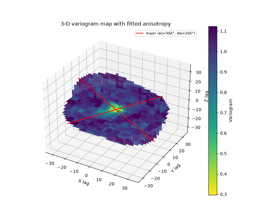
plot_map3d uses the cached raw cloud and draws a horizontal lag slice plus a vertical fence aligned with the fitted model azimuth. This is a quick visual check that the selected model direction follows the low-variogram continuity.

fig = plt.figure(figsize=(8.5, 7.0))
ax = fig.add_subplot(111, projection="3d")
model.plot_map3d(
    ax=ax,
    cutoff=36.0,
    dx=2.0,
    dy=2.0,
    dz=2.0,
    fill_nan=True,  # display-only nearest fill to avoid checkerboard gaps
    # n_fences=3,
    title="3-D variogram map with fitted anisotropy",
)
plt.show()

Plot the directional variograms and the fitted model

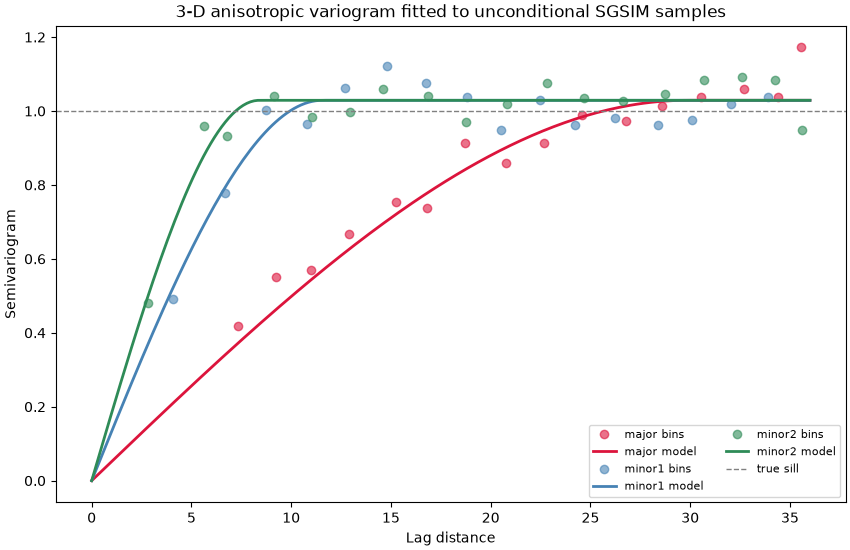
Each axis is evaluated along its own unit direction with calc_variogram(), which applies the full 3-D anisotropy, so the three model curves reach the sill at their respective ranges.

COLORS = {"major": "crimson", "minor1": "steelblue", "minor2": "seagreen"}

# Unit direction vector for each principal axis from the fixed orientation.
# rotation_matrix_3d returns columns ordered (major, minor1, minor2).
names = ["major", "minor1", "minor2"]
directions = rotation_matrix_3d(TRUE["azimuth"], TRUE["dip"], TRUE["plunge"]).T

fig, ax = plt.subplots(figsize=(8.5, 5.5), layout="constrained")
for j, name in enumerate(names):
    sub = dir_avg.loc[dir_avg["axis"] == name]
    ax.plot(sub["lag"], sub["variogram"], "o", color=COLORS[name],
            alpha=0.6, label=f"{name} bins")
    h = np.linspace(0.0, 36.0, 200)
    coord0 = np.zeros((len(h), 3))
    coord1 = directions[j] * h[:, None]
    ax.plot(h, model.calc_variogram(coord0, coord1), color=COLORS[name], lw=2,
            label=f"{name} model")

ax.axhline(TRUE["sill"], color="0.5", ls="--", lw=1.0, label="true sill")
ax.set_xlabel("Lag distance")
ax.set_ylabel("Semivariogram")
ax.set_title("3-D anisotropic variogram fitted to unconditional SGSIM samples")
ax.legend(fontsize=8, ncol=2)
plt.show()