Spatially varying anisotropy (SVA)

Case study: coarse-fraction interpolation in the Sacramento River alluvial aquifer, Butte County, CA (west of Chico).

In a meandering river system sediments are elongated along the active channel belt, so the variogram major axis should follow the local channel bearing — which rotates as the river meanders across the domain. A single global anisotropy cannot capture this geometry. Spatially varying anisotropy (SVA) assigns an independent variogram to every prediction block, whose major axis tracks the local channel orientation at that block.

Workflow (adapted from the GMDSI conceptual-SVA tutorial, Doherty 2018):

1. Assign local anisotropy — each observation well is assigned a local azimuth and estimated correlation ranges from the nearest mapped river channel segment (columns azimuth, a_major, a_minor in pc2d.csv).

2. Bootstrap the variogram field — krige azimuth, major range, and anisotropy ratio from the wells onto every grid node using two successive iterations. The helper variogram for iteration 1 is the SVA field produced by iteration 0, which better honours the channel-parallel spatial structure.

3. Compare three models — isotropic, global anisotropy (fixed azimuth), and SVA — by visual inspection and leave-one-out cross-validation.

Data files

pc2d.csv

62 percent-coarse measurements with pre-assigned local azimuth, a_major, and a_minor for each well.

grid2d.csv

4 800-node (80 × 60) prediction grid in UTM Zone 10N (metres).

river_butte.csv

Digitised Sacramento River channel segments in grid row/column coordinates, used for map overlays.

import numpy as np
import pandas as pd
import matplotlib.pyplot as plt
from mpl_toolkits.axes_grid1 import ImageGrid
from krigekit import Kriging


# ---------------------------------------------------------------------------
# Variogram parameters — spherical model, coarse fraction (unitless, 0–1)
# ---------------------------------------------------------------------------
SILL, NUGGET = 0.12, 0.0
A_MAJOR, A_MINOR = 8000.0, 2000.0   # global-anisotropy baseline ranges (m)
A_ISO = 5000.0                      # isotropic reference range (m)
NMAX = 30                           # maximum neighbourhood size

GRID_SHAPE = (80, 60)               # rows × cols of the prediction grid
ROTATION = 35                       # grid bearing from north (degrees CW)

# ---------------------------------------------------------------------------
# Load data
# ---------------------------------------------------------------------------
obs   = pd.read_csv("../../test_data/pc2d.csv")
grid  = pd.read_csv("../../test_data/grid2d.csv")
river = pd.read_csv("../../test_data/river_butte.csv")

oc = obs[["x", "y"]].to_numpy(float)   # observation coordinates
ov = obs["pc"].to_numpy(float)          # observed coarse fraction
gc = grid[["x", "y"]].to_numpy(float)  # grid coordinates


# ---------------------------------------------------------------------------
# Kriging helpers
# ---------------------------------------------------------------------------
def krige_sva(oc, ov, gc, gaz, gamaj, gamin):
    """Krige *ov* onto *gc* with a per-block SVA variogram."""
    k = Kriging(ndim=2, nvar=1, varying_vgm=True)
    k.set_obs(ivar=1, coord=oc, value=ov)
    k.set_grid(coord=gc)
    for ib in range(len(gaz)):
        k.set_vgm_block(ib + 1, 1, 1, vtype="sph", nugget=NUGGET, sill=SILL,
                        a_major=float(gamaj[ib]), a_minor1=float(gamin[ib]),
                        azimuth=float(gaz[ib]))
    k.set_search(ivar=1, nmax=NMAX)
    k.solve()
    est, var = k.get_results()
    del k
    return np.ravel(np.asarray(est)), np.ravel(np.asarray(var))


def krige_global(oc, ov, gc, vgm):
    """Krige *ov* onto *gc* with a single stationary variogram *vgm*."""
    k = Kriging(ndim=2, nvar=1)
    k.set_obs(ivar=1, coord=oc, value=ov)
    k.set_vgm(ivar=1, jvar=1, **vgm)
    k.set_grid(coord=gc)
    k.set_search(ivar=1, nmax=NMAX)
    k.solve()
    est, var = k.get_results()
    del k
    return np.ravel(np.asarray(est)), np.ravel(np.asarray(var))


def krige_cv_global(oc, ov, vgm):
    """Leave-one-out cross-validation with a stationary variogram."""
    k = Kriging(ndim=2, nvar=1, cross_validation=True)
    k.set_obs(ivar=1, coord=oc, value=ov)
    k.set_vgm(ivar=1, jvar=1, **vgm)
    k.set_grid_cv()
    k.set_search(ivar=1)
    k.solve()
    est, var = k.get_results()
    del k
    return np.ravel(np.asarray(est)), np.ravel(np.asarray(var))


def krige_cv_sva(oc, ov, az_obs, am_obs, amin_obs):
    """Leave-one-out cross-validation with per-observation SVA variogram.

    In LOO-CV mode the prediction locations are the observation points
    themselves, so each ``set_vgm_block`` call receives the local azimuth
    and ranges already assigned to that well.
    """
    k = Kriging(ndim=2, nvar=1, cross_validation=True, varying_vgm=True)
    k.set_obs(ivar=1, coord=oc, value=ov)
    k.set_grid_cv()
    for ib in range(len(az_obs)):
        k.set_vgm_block(ib + 1, 1, 1, vtype="sph", nugget=NUGGET, sill=SILL,
                        a_major=float(am_obs[ib]), a_minor1=float(amin_obs[ib]),
                        azimuth=float(az_obs[ib]))
    k.set_search(ivar=1)
    k.solve()
    est, var = k.get_results()
    del k
    return np.ravel(np.asarray(est)), np.ravel(np.asarray(var))


def to_2d(v):
    """Reshape a flat grid vector to a 2-D image array."""
    return np.asarray(v).reshape(GRID_SHAPE)


def to_less(v, step=5):
    """Sub-sample a flat grid vector for sparse quiver overlays."""
    i0 = step // 2
    return np.asarray(v).reshape(GRID_SHAPE)[i0::step, i0::step].flatten()


def plot_grid_az(ax, gaz):
    """Overlay anisotropy-direction arrows on a grid-index image."""
    L = 2
    xc, yc = np.meshgrid(range(GRID_SHAPE[1]), range(GRID_SHAPE[0]))
    xc = to_less(xc.flatten())
    yc = to_less(yc.flatten())
    a  = np.deg2rad(to_less(gaz) + ROTATION)
    ux, uy = np.sin(a) * L, np.cos(a) * L
    ax.quiver(xc, yc, ux, -uy, angles="xy", scale_units="xy", zorder=3)


def plot_riv_grid(ax, color="#4a90d9", lw=1.0, zorder=1, **kw):
    """Overlay digitised river channels on a grid-index image."""
    for _, df in river.groupby("segment"):
        ax.plot(df["column"] - 0.5, df["row"] - 0.5,
                color=color, lw=lw, zorder=zorder, **kw)

Observations — local anisotropy at each well

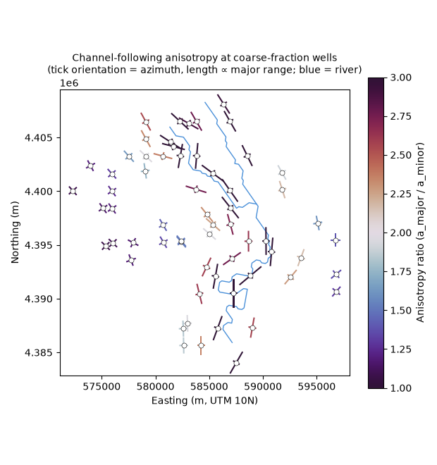
Each well was assigned a local anisotropy azimuth (the bearing of the nearest mapped river channel segment) and estimated correlation ranges (major axis along the channel, minor axis perpendicular to it).

The quiver plot below shows the major-axis orientation as a tick mark at each well. Tick length is proportional to the major range; colour encodes the anisotropy ratio a_major / a_minor.

scale = 0.17

fig, ax = plt.subplots(figsize=(6.2, 6.6))
for _, df in river.groupby("segment"):
    ax.plot(df["x"], df["y"], color="#4a90d9", lw=1.0, zorder=1)

# minor arm of the tick (perpendicular direction, +90°)
az_rad = np.radians(obs["azimuth"] + 90)
L = obs["a_minor"] * scale
ux, uy = np.sin(az_rad) * L, np.cos(az_rad) * L
ax.quiver(obs["x"], obs["y"], ux, uy, obs["a_major"] / obs["a_minor"],
          angles="xy", scale_units="xy", scale=0.5,
          headwidth=0, headlength=0, headaxislength=0, pivot="mid",
          width=0.005, cmap="twilight_shifted", clim=(1.0, 3.0), zorder=3)

# major arm of the tick (along-channel direction)
az_rad = np.radians(obs["azimuth"])
L = obs["a_major"] * scale
ux, uy = np.sin(az_rad) * L, np.cos(az_rad) * L
q = ax.quiver(obs["x"], obs["y"], ux, uy, obs["a_major"] / obs["a_minor"],
              angles="xy", scale_units="xy", scale=0.5,
              headwidth=0, headlength=0, headaxislength=0, pivot="mid",
              width=0.005, cmap="twilight_shifted", clim=(1.0, 3.0), zorder=4)
ax.scatter(obs["x"], obs["y"], facecolors="white", s=26,
           edgecolors="k", linewidths=0.4, zorder=4)
plt.colorbar(q, ax=ax, shrink=0.7, label="Anisotropy ratio (a_major / a_minor)")
ax.set_aspect("equal")
ax.set_xlabel("Easting (m, UTM 10N)")
ax.set_ylabel("Northing (m)")
ax.set_title("Channel-following anisotropy at coarse-fraction wells\n"
             "(tick orientation = azimuth, length ∝ major range; blue = river)",
             fontsize=10)
fig.tight_layout()
plt.show()

Bootstrap the variogram field — two iterations

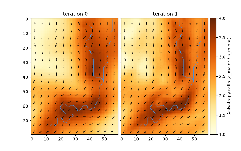
SVA kriging requires azimuth and range values at every grid node before the main interpolation run. We obtain them by kriging the per-well anisotropy attributes (azimuth, major range, anisotropy ratio) onto the grid.

Iteration 0 uses an isotropic helper variogram (range = A_ISO) to produce a first-pass SVA field over the entire grid.

Iteration 1 re-kriges the same well attributes using the SVA field from iteration 0 as the helper variogram, refining the spatial structure along the channel corridor.

Note

Azimuth is shifted by +360° before kriging to avoid wrap-around discontinuities near 0°/360°. The offset is subtracted afterwards.

vgm_iso = dict(vtype="sph", nugget=NUGGET, sill=SILL, a_major=A_ISO)

# iteration 0: isotropic helper
vgm_iter0 = {}
vgm_iter0["az"], _ = krige_global(oc, obs["azimuth"] + 360, gc, vgm_iso)
vgm_iter0["az"] -= 360
vgm_iter0["am"], _ = krige_global(oc, obs["a_major"],               gc, vgm_iso)
vgm_iter0["an"], _ = krige_global(oc, obs["a_major"] / obs["a_minor"], gc, vgm_iso)
vgm_iter0["a2"] = vgm_iter0["am"] / np.maximum(1.0, vgm_iter0["an"])

# iteration 1: SVA helper derived from iteration 0
vgm_iter1 = {}
vgm_iter1["az"], _ = krige_sva(oc, obs["azimuth"] + 360, gc,
                                vgm_iter0["az"], vgm_iter0["am"], vgm_iter0["a2"])
vgm_iter1["az"] -= 360
vgm_iter1["am"], _ = krige_sva(oc, obs["a_major"], gc,
                                vgm_iter0["az"], vgm_iter0["am"], vgm_iter0["a2"])
vgm_iter1["an"], _ = krige_sva(oc, obs["a_major"] / obs["a_minor"], gc,
                                vgm_iter0["az"], vgm_iter0["am"], vgm_iter0["a2"])
vgm_iter1["a2"] = vgm_iter1["am"] / np.maximum(1.0, vgm_iter1["an"])

fig = plt.figure(figsize=(8, 5))
axs = ImageGrid(fig, 111, nrows_ncols=(1, 2), axes_pad=0.1,
                label_mode="L", cbar_mode="single", cbar_size="7%", cbar_pad="2%")
for ax, vgm, label in zip(axs, [vgm_iter0, vgm_iter1], ["Iteration 0", "Iteration 1"]):
    im = ax.imshow(to_2d(vgm["an"]), vmin=1, vmax=4, cmap="YlOrBr")
    plot_grid_az(ax, vgm["az"])
    plot_riv_grid(ax, zorder=10)
    ax.set(title=label)
axs.cbar_axes[0].colorbar(im, label="Anisotropy ratio (a_major / a_minor)")
plt.show()

Krige coarse fraction — three models

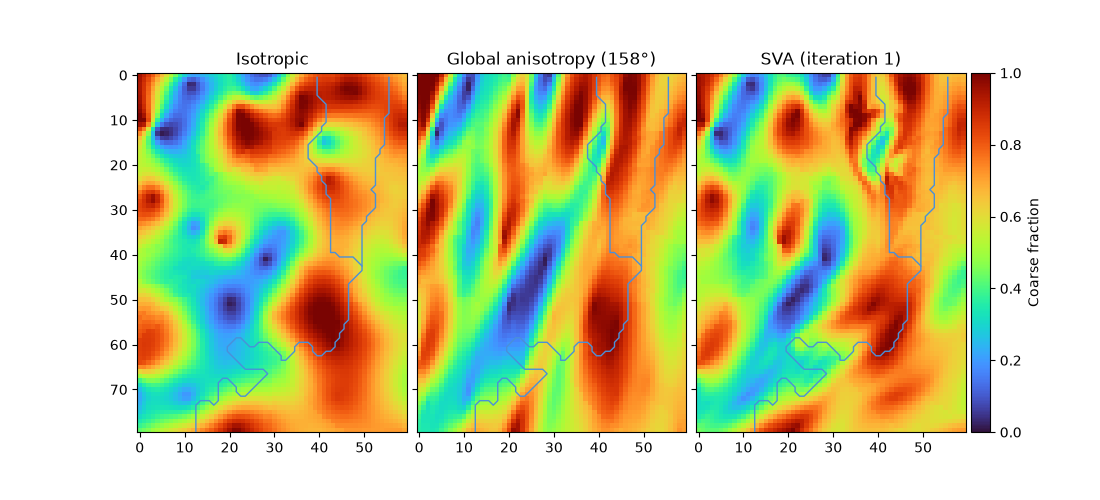
Three ordinary-kriging runs interpolate percent-coarse onto the prediction grid:

• Isotropic — spherical, range = A_ISO = 5 000 m, no preferred direction.

• Global anisotropy — spherical, major range = A_MAJOR = 8 000 m, minor range = A_MINOR = 2 000 m, azimuth fixed at 158° (representative channel bearing at domain centre).

• SVA (iteration 1) — same sill/nugget, but each grid block uses its own azimuth and ranges from the bootstrapped variogram field above.

VGM_ISO = dict(vtype="sph", nugget=NUGGET, sill=SILL, a_major=A_ISO)
VGM_GLB = dict(vtype="sph", nugget=NUGGET, sill=SILL,
               a_major=A_MAJOR, a_minor1=A_MINOR, azimuth=158)

est_iso,  _ = krige_global(oc, ov, gc, VGM_ISO)
est_glb,  _ = krige_global(oc, ov, gc, VGM_GLB)
est_sva1, _ = krige_sva(oc, ov, gc,
                         vgm_iter1["az"], vgm_iter1["am"], vgm_iter1["a2"])

model_labels = ["Isotropic", "Global anisotropy (158°)", "SVA (iteration 1)"]
estimates    = [est_iso, est_glb, est_sva1]

fig = plt.figure(figsize=(11, 5))
axs = ImageGrid(fig, 111, nrows_ncols=(1, 3), axes_pad=0.1,
                label_mode="L", cbar_mode="single", cbar_size="7%", cbar_pad="2%")
for ax, est, label in zip(axs, estimates, model_labels):
    im = ax.imshow(to_2d(est), vmin=0, vmax=1, cmap="turbo")
    plot_riv_grid(ax, zorder=10)
    ax.set(title=label)
axs.cbar_axes[0].colorbar(im, label="Coarse fraction")
plt.show()

Leave-one-out cross-validation

LOO-CV predicts each well from its neighbours (leaving it out of the kriging system) and returns one estimate and one variance per observation. Two diagnostics quantify model performance:

• RMSE — root-mean-squared prediction error (lower is better).

• MSSE — mean standardised squared error = mean((z − ẑ)² / σ²). A well-calibrated model gives MSSE ≈ 1; MSSE > 1 means the variogram underestimates prediction uncertainty.

def cv_stats(obs_v, est_cv, var_cv):
    res  = obs_v - est_cv
    rmse = np.sqrt(np.mean(res ** 2))
    msse = np.mean(res ** 2 / var_cv)
    r    = np.corrcoef(obs_v, est_cv)[0, 1]
    return rmse, msse, r


est_cv_iso, var_cv_iso = krige_cv_global(oc, ov, VGM_ISO)
est_cv_glb, var_cv_glb = krige_cv_global(oc, ov, VGM_GLB)
est_cv_sva, var_cv_sva = krige_cv_sva(oc, ov,
                                       obs["azimuth"].to_numpy(float),
                                       obs["a_major"].to_numpy(float),
                                       obs["a_minor"].to_numpy(float))

cv_results = [
    ("Isotropic",         est_cv_iso, var_cv_iso),
    ("Global anisotropy", est_cv_glb, var_cv_glb),
    ("SVA",               est_cv_sva, var_cv_sva),
]

print(f"{'Model':<26}  {'RMSE':>7}  {'MSSE':>6}  {'r':>6}")
for label, est_cv, var_cv in cv_results:
    rmse, msse, r = cv_stats(ov, est_cv, var_cv)
    print(f"{label:<26}  {rmse:>7.4f}  {msse:>6.2f}  {r:>6.3f}")

fig, axes = plt.subplots(1, 3, figsize=(14, 4.5), sharey=True,
                         gridspec_kw={"wspace": 0.3})
for ax, (label, est_cv, var_cv) in zip(axes, cv_results):
    rmse, msse, r = cv_stats(ov, est_cv, var_cv)
    ax.scatter(ov, est_cv, s=50, edgecolors="k", linewidths=0.35, alpha=0.85)
    ax.plot([0, 1], [0, 1], "r--", lw=1.2, label="1:1 line")
    ax.set_xlim(0, 1); ax.set_ylim(0, 1)
    ax.set_xlabel("Observed (coarse fraction)")
    ax.set_title(f"{label}\nr = {r:.3f},  RMSE = {rmse:.4f},  MSSE = {msse:.2f}")
    ax.legend(fontsize=9)
axes[0].set_ylabel("LOO-CV estimate")
plt.show()

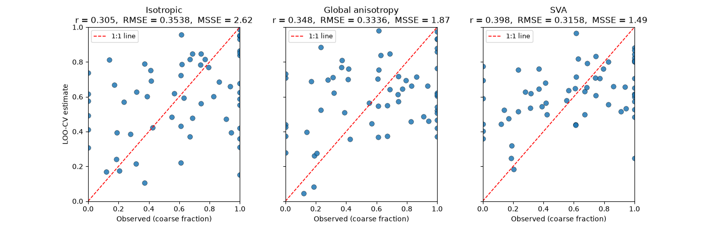
Model                          RMSE    MSSE       r
Isotropic                    0.3538    2.62   0.305
Global anisotropy            0.3336    1.87   0.348
SVA                          0.3158    1.49   0.398