Space-time kriging — CCl4 plume

Groundwater contamination by carbon tetrachloride (CCl4) . The dataset covers 281 monitoring wells sampled at irregular intervals from 2008 to 2020, yielding 4 512 observations distributed across both space (~10 km domain) and time (~13 years).

This example walks through the first step of a space-time kriging workflow: computing and visualising the empirical space-time variogram cloud. In a space-time variogram every pair of observations (i, j) contributes one point:

\[\gamma_{ij} = \tfrac{1}{2}(z_i - z_j)^2\]

plotted at spatial lag \(h_s = \|\mathbf{x}_i - \mathbf{x}_j\|\) (metres) and temporal lag \(h_t = |t_i - t_j|\) (years).

CCl4 concentrations span three orders of magnitude (0.04–5 900 µg/L). A uniform quantile transform is applied before computing the variogram: ranks are mapped to percentiles on [0, 1], suppressing outlier influence without assuming a specific parametric distribution such as log-normal. The dedicated st_variogram_fitting_ctet.py example uses SpaceTimeVariogramModel for the full spatial-temporal lag surface, product-sum fitting, and manual-adjustment workflow.

import time
import numpy as np
import pandas as pd
import matplotlib.pyplot as plt
from scipy.optimize import minimize
from sklearn.preprocessing import QuantileTransformer
from krigekit import SpaceTimeKriging


# ---------------------------------------------------------------------------
# Constants
# ---------------------------------------------------------------------------
MAX_HS = 5_500      # spatial lag cutoff for variogram cloud display (m)
MAX_HT = 13         # temporal lag cutoff (years)
MINCNT = 5          # minimum pairs per hexbin cell before displaying

Heler functions

def plot_3d(
    nrow=1,
    ncol=1,
    vs=None,
    figsize=(8, 8),
    cmap=plt.get_cmap("jet"),
    titles=None,
    dx=500,
    dy=0.5,
):
    if vs is None:
        vs = []
    if titles is None:
        titles = [""] * len(vs)

    fig, axs = plt.subplots(
        nrow,
        ncol,
        figsize=figsize,
        subplot_kw={"projection": "3d"},
        sharex=True,
        sharey=True,
        tight_layout=True,
    )

    axs = np.atleast_1d(axs).ravel()

    # Global z/color range, so all subplots are comparable
    all_values = np.concatenate([v.values.ravel() for v in vs])
    vmin = np.nanquantile(all_values, 0.01)
    vmax = np.nanquantile(all_values, 0.99)

    if np.isclose(vmax, vmin):
        vmax = vmin + 1e-12

    norm = plt.Normalize(vmin=vmin, vmax=vmax)

    xmins, xmaxs, ymins, ymaxs, zmaxs = [], [], [], [], []

    for ax, v, title in zip(axs, vs, titles):
        X, Y = np.meshgrid(v.columns, v.index)
        Z = v.values

        colors = cmap(norm(Z.ravel()))

        ax.bar3d(
            X.ravel(),
            Y.ravel(),
            np.zeros(Z.size),
            dx,
            dy,
            Z.ravel(),
            shade=True,
            color=colors,
            edgecolor="w",
        )

        ax.set(
            xlabel="Spatial lag $h_s$ (m)",
            ylabel="Temporal lag $h_t$ (years)",
            title=title,
        )

        ax.view_init(20, -154)

        xmins.append(np.nanmin(X))
        xmaxs.append(np.nanmax(X) + dx)
        ymins.append(np.nanmin(Y))
        ymaxs.append(np.nanmax(Y) + dy)
        zmaxs.append(np.nanmax(Z))

    # Sync all axes
    for ax in axs:
        ax.set_xlim(min(xmins), max(xmaxs))
        ax.set_ylim(min(ymins), max(ymaxs))
        ax.set_zlim(0, max(zmaxs))

    # Hide unused axes if vs has fewer panels
    for ax in axs[len(vs):]:
        ax.set_visible(False)

    return fig, axs

Load data and convert time to decimal year

Time is stored as month/day/year hour:minute strings. We convert to decimal year as year + day_of_year / 365, so 31 January 2005 becomes 2005 + 31/365 ≈ 2005.085.

CCl4 is then transformed to uniform quantile scores using QuantileTransformer. The fitted transformer qt is stored for back-transformation after kriging.

df = pd.read_csv("../../test_data/ctet.csv")
df["datetime"] = pd.to_datetime(df["time"], format="%m/%d/%Y %H:%M").dt.date
df["t"] = df["datetime"].apply(
    lambda dt: dt.year + dt.timetuple().tm_yday / 365
)
df = df.groupby(["well", "x","y","z","t"], as_index=False)["CCl4"].mean()
qt = QuantileTransformer(output_distribution="uniform", random_state=0)
df["uscore"] = qt.fit_transform(df[["CCl4"]]).ravel()

print(f"Observations : {len(df):,}")
print(f"Wells        : {df['well'].nunique()}")
print(f"Time range   : {df['t'].min():.3f} – {df['t'].max():.3f}")
print(f"CCl4 range   : {df['CCl4'].min():.3g} – {df['CCl4'].max():.3g} µg/L")
print(f"Uniform score: {df['uscore'].min():.2f} – {df['uscore'].max():.2f}")

Observations : 3,823
Wells        : 281
Time range   : 2008.008 – 2020.997
CCl4 range   : 0.042 – 5.9e+03 µg/L
Uniform score: 0.00 – 1.00

Spatial and temporal overview

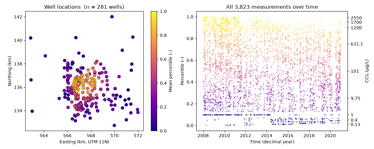
Well locations coloured by time-averaged uniform score (left), and all measurements plotted over time coloured by uniform score (right).

mean_by_well = df.groupby("well").agg(
    x=("x", "first"), y=("y", "first"), uscore=("uscore", "mean")
).reset_index()

fig, axes = plt.subplots(1, 2, figsize=(12, 4.8))

ax = axes[0]
sc = ax.scatter(mean_by_well["x"] / 1000, mean_by_well["y"] / 1000,
                c=mean_by_well["uscore"], cmap="plasma",
                vmin=0, vmax=1, s=55, edgecolors="k", linewidths=0.35)
plt.colorbar(sc, ax=ax, label="Mean percentile (–)")
ax.set_xlabel("Easting (km, UTM 11N)")
ax.set_ylabel("Northing (km)")
ax.set_title(f"Well locations  (n = {len(mean_by_well)} wells)")
ax.set_aspect("equal")

ax = axes[1]
sc2 = ax.scatter(df["t"], df["uscore"],
                 c=df["uscore"], cmap="plasma",
                 vmin=0, vmax=1, s=6, alpha=0.6, linewidths=0)
ax.set_xlabel("Time (decimal year)")
ax.set_ylabel("Percentile (–)")
ax.set_title(f"All {len(df):,} measurements over time")

# --------------------------------------------------
# Secondary axis showing native CCl4 concentrations
# --------------------------------------------------
ax2 = ax.twinx()

# Use the same percentile scale
ax2.set_ylim(ax.get_ylim())

# Choose percentile locations for ticks
p_ticks = np.array([0.01, 0.05, 0.10, 0.25,
                    0.50, 0.75, 0.90, 0.95, 0.99])

# Convert percentiles back to concentration
c_ticks = qt.inverse_transform(
    p_ticks.reshape(-1, 1)
).ravel()

ax2.set_yticks(p_ticks)
ax2.set_yticklabels([f"{v.round(2):.4g}" for v in c_ticks])

ax2.set_ylabel("CCl₄ (µg/L)")

fig.tight_layout()
plt.show()

Compute empirical variogram cloud

All ~10 million pairs are evaluated; distance cutoff is at 5500 approximate plume downstream length. only wells with 6+ measurements are used.

The spatial lag is computed in 3-D (x, y, z) with z scaled by Z_SCALE = 5 to account for vertical anisotropy — a first-attempt value that can be tuned once the variogram structure is clearer.

dm = df.groupby('well').uscore.count().sort_values()
ws = dm[dm>6].index.values
mask = df.well.isin(ws)
Z_SCALE = 5  # vertical anisotropy factor (first attempt)
X = np.column_stack([df.loc[mask, "x"], df.loc[mask, "y"], df.loc[mask, "z"] * Z_SCALE])
T = df.loc[mask, "t"].to_numpy(float)
V = df.loc[mask, "uscore"].to_numpy(float)

i_idx, j_idx = np.triu_indices(mask.sum(), k=1)

hs    = np.sqrt(np.sum((X[i_idx] - X[j_idx]) ** 2, axis=1))  # 3-D spatial lag (m, z scaled ×5)
ht    = np.abs(T[i_idx] - T[j_idx])                           # temporal lag (yr)
gamma = 0.5 * (V[i_idx] - V[j_idx]) ** 2                     # semi-variance

mask2 = (hs <= MAX_HS) & (ht <= MAX_HT)
hs = hs[mask2]; ht = ht[mask2]; gamma = gamma[mask2]
print(f"Total pairs : {len(hs):,}")
print(f"h_s range   : {hs.min():.1f} – {hs.max():.1f} m")
print(f"h_t range   : {ht.min():.3f} – {ht.max():.3f} yr")
print(f"γ range     : {gamma.min():.3f} – {gamma.max():.3f}")

Total pairs : 6,320,157
h_s range   : 0.0 – 5498.3 m
h_t range   : 0.000 – 12.989 yr
γ range     : 0.000 – 0.499

Average (experimental) variogram

Pairs are binned by spatial lag (500 m intervals) and temporal lag (0.5-year intervals). Each bin reports the mean semi-variance and the pair count; bins with fewer than MINCNT pairs are dropped.

The result is a 2-D table indexed by (h_s centre, h_t centre) and can be inspected as a heat map or as 1-D slices for model fitting.

HS_STEP = 500       # spatial bin width (m)
HT_STEP = 0.5       # temporal bin width (years)

# bin indices (0-based)
hs_bin = (hs / HS_STEP).astype(int)
ht_bin = (ht / HT_STEP).astype(int)

# aggregate with pandas groupby
pairs = pd.DataFrame({
    "hs_bin": hs_bin, "ht_bin": ht_bin,
    "hs":hs ,"ht":ht, "gamma": gamma})
vgm = (pairs.groupby(["hs_bin", "ht_bin"])["gamma"]
             .agg(gamma_mean="mean", n_pairs="count"))
hst = pairs.groupby(["hs_bin", "ht_bin"])[["hs", "ht"]].mean()
vgm = pd.merge(vgm, hst, on=["hs_bin", "ht_bin"]).reset_index()
vgm = vgm[vgm["n_pairs"] >= MINCNT].copy()

# convert bin indices back to lag-centre values
vgm["hs_m"]  = (vgm["hs_bin"] + 0.5) * HS_STEP   # metres
vgm["ht_yr"] = (vgm["ht_bin"] + 0.5) * HT_STEP   # years

print(f"Occupied bins : {len(vgm):,}")
print(vgm[["hs_m", "ht_yr", "gamma_mean", "n_pairs"]].head(12).to_string(index=False))

Occupied bins : 286
 hs_m  ht_yr  gamma_mean  n_pairs
250.0   0.25    0.031859    49243
250.0   0.75    0.031499    43069
250.0   1.25    0.031143    40313
250.0   1.75    0.030192    33855
250.0   2.25    0.029131    31144
250.0   2.75    0.027890    25950
250.0   3.25    0.028102    24403
250.0   3.75    0.029527    21483
250.0   4.25    0.029790    19788
250.0   4.75    0.030256    19346
250.0   5.25    0.033310    18676
250.0   5.75    0.034687    18353

Fit product-sum space-time variogram

The product-sum model (De Cesare et al., 2001) expressed in terms of marginals normalised to unit sill:

\[\gamma(h_s, h_t) = a\,\tilde\gamma_S(h_s) + b\,\tilde\gamma_T(h_t) + p\,\tilde\gamma_S(h_s)\,\tilde\gamma_T(h_t)\]

The cross-term coefficient \(p\) is constrained to \(p \le 0\). A negative \(p\) corresponds to a positive coupling coefficient \(k_\text{ps}\) in the krigekit covariance form (\(k_\text{ps} = -p / (C_S(0) C_T(0))\)), meaning observations that are close in both space and time are more correlated than the two marginals alone would predict. This is the physically appropriate behaviour for a coherent, slowly evolving groundwater plume and matches the original De Cesare et al. (2001) convention of \(k \ge 0\). Validity requires \(a, b > 0\) and \(a + b + p > 0\) (positive total sill). Uniform-score variance is approximately \(1/12\); the fitted product-sum coefficients need not sum to one.

Parameters are optimised by weighted least squares over all occupied (h_s, h_t) bins, with weights proportional to pair count.

# Why Gaussian: the CCl4 plume is a coherent, slowly-evolving body —
# concentration at a location is smoothly autocorrelated in time over years.
# Spherical/exponential decay too steeply near the origin and throw away that
# multi-year temporal coherence; the Gaussian's flat-then-smooth shape matches
# the physics, which is exactly why it predicts the held-out observations best.

def sph_model(h, nugget, sill, a):
    """Spherical variogram: γ(0) = 0, plateau at nugget + sill for h ≥ a."""
    h = np.asarray(h, float)
    g = np.full_like(h, nugget + sill)
    m = (h > 0) & (h < a)
    g[m] = nugget + sill * (1.5 * (h[m] / a) - 0.5 * (h[m] / a) ** 3)
    g[h == 0] = 0.0
    return g


def gauss_model(h, nugget, sill, a):
    """Gaussian variogram: γ(h) = nugget + sill·(1 − exp(−3h²/a²)); a = practical range."""
    h = np.asarray(h, float)
    g = nugget + sill * (1.0 - np.exp(-3.0 * (h / a) ** 2))
    g[h == 0] = 0.0
    return g


def gs(hs, a_s):
    """Spatial marginal normalised to sill = 1."""
    return sph_model(hs, 0.0, 1.0, a_s)


def gt(ht, a_t):
    """Temporal marginal (Gaussian) normalised to sill = 1."""
    return gauss_model(ht, 0.0, 1.0, a_t)


def gamma_ps(hs, ht, a, b, p, a_s, a_t):
    return (a * gs(hs, a_s) + b * gt(ht, a_t) +
            p * gs(hs, a_s) *     gt(ht, a_t))


hs_all = vgm["hs_m"].values
ht_all = vgm["ht_yr"].values
gm_all = vgm["gamma_mean"].values

w_all  = vgm["n_pairs"].rank()
w_all = 1.01**np.where(w_all<w_all.mean(), w_all.max()-w_all, w_all)
w_all = vgm["gamma_mean"].values
w_all = vgm["n_pairs"].values

def wls_obj(params):
    a, b, p, a_s, a_t = params
    if a < 0 or b < 0 or a_s < 0 or a_t < 0:
        return 1e12
    if p > 0 or a + b + p <= 0:   # p ≤ 0; total sill must stay positive
        return 1e12
    pred = gamma_ps(hs_all, ht_all, a, b, p, a_s, a_t)
    return float(np.sum(w_all * (pred - gm_all) ** 2))


res = minimize(wls_obj, x0=[0.11, 0.025, -0.01, 2500, 6.5], method="Nelder-Mead",
               options={"xatol": 1e-7, "fatol": 1e-10, "maxiter": 20000})


a_ps, b_ps, p_ps, a_s, a_t = res.x
print( "Product-sum fit:")
print(f"  a = {a_ps:.4f}  (spatial contribution)")
print(f"  b = {b_ps:.4f}  (temporal contribution)")
print(f"  p = {p_ps:.4f}  (coupling strength)")
print(f"a_s = {a_s :.4f}  (spatial range)")
print(f"a_t = {a_t :.4f}  (temporal range)")
print(f"  total sill = {a_ps + b_ps + p_ps:.4f}  (target ≈ 1, p ≤ 0)")

Product-sum fit:
  a = 0.1076  (spatial contribution)
  b = 0.0206  (temporal contribution)
  p = -0.0133  (coupling strength)
a_s = 3413.8512  (spatial range)
a_t = 0.0580  (temporal range)
  total sill = 0.1148  (target ≈ 1, p ≤ 0)

3D Heat map of the experimental and fitted variogram

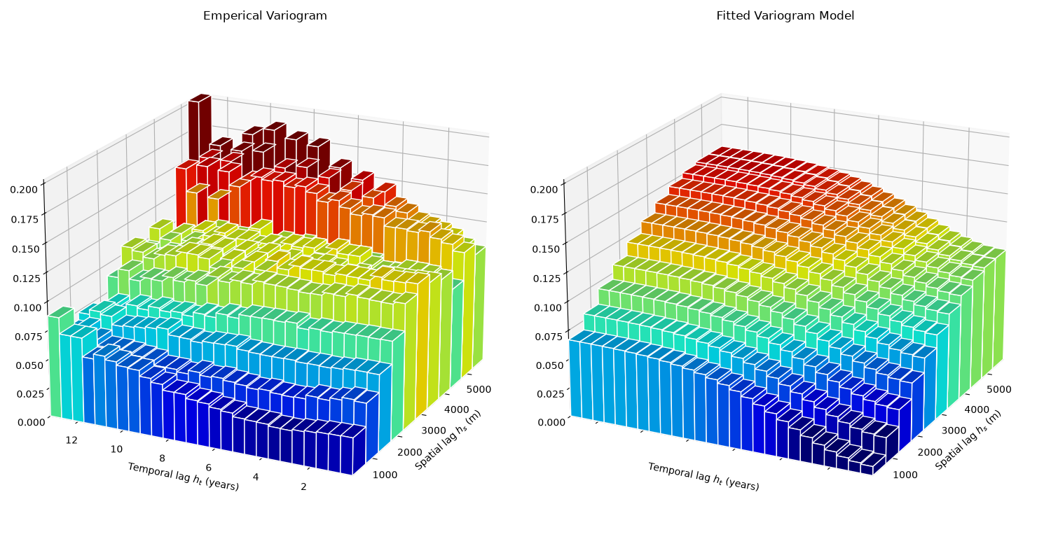
The experimental variogram surface plotted on the (h_s, h_t) grid. Temporal slices (rows of constant h_t) will be used for model fitting in the next step. The variogram parameters are manually adjusted. See st_variogram_fitting_ctet.py for the SpaceTimeVariogramModel constrained multistart fit, identifiability diagnostics, and automatic-versus-production comparison.

a_ps = 0.10
b_ps = 0.06
p_ps = -0.005
a_s  = 5000
a_t  = 9
v = vgm.pivot(columns="hs_m", index="ht_yr", values="gamma_mean").loc[:,:5500]
X, Y = np.meshgrid(v.columns, v.index)
v_fit = v.copy()
v_fit[:] = gamma_ps(X, Y, a_ps, b_ps, p_ps, a_s, a_t)
plot_3d(nrow=1, ncol=2, vs=[v, v_fit], figsize=(15,8), cmap=plt.get_cmap('jet'),
        titles=["Emperical Variogram", "Fitted Variogram Model"])
plt.show()

Space-time ordinary kriging

Load the structured 3-D spatial grid from the ESRI ASCII elevation rasters, then convert the fitted product-sum variogram coefficients to krigekit’s covariance parameterisation and run ordinary space-time kriging at six biennial time snapshots (mid-year, t = year + 0.5).

Variogram → covariance conversion

krigekit stores the product-sum model as a covariance:

\[C(h_s, h_t) = k_\text{ps}\,C_S(h_s)\,C_T(h_t) + C_S(h_s) + C_T(h_t)\]

Expanding \(\gamma = C(0,0) - C(h_s,h_t)\) and collecting terms in \(\tilde\gamma_S, \tilde\gamma_T\) (normalised marginals, sill = 1) yields three matching equations. Solving for the three unknowns gives:

\[C_S(0) = a + p, \qquad C_T(0) = b + p, \qquad k_\text{ps} = -\frac{p}{C_S(0)\cdot C_T(0)}\]

Because \(p < 0\), the marginal sills \(C_S(0) < a\) and \(C_T(0) < b\), and \(k_\text{ps} > 0\) — the De Cesare convention that rewards space-time proximity.

Temporal search scale time_at

The KD-tree neighbour search operates in the combined \((x, y, z, t \cdot \text{time\_at})\) space, so time_at must convert years into metres. Requiring that a unit displacement in each dimension causes equal covariance loss:

\[\underbrace{\frac{C_S(0)}{a_s}}_{\text{spatial rate}} = \text{time\_at} \times \underbrace{\frac{C_T(0)}{a_t}}_{\text{temporal rate}} \;\Longrightarrow\; \text{time\_at} = \frac{a_s}{a_t} \cdot \frac{C_S(0)}{C_T(0)}\]

The naive value \(a_s / a_t\) treats both marginals as equally important; the sill correction \(C_S(0)/C_T(0)\) weights time down when the temporal variogram explains proportionally less variance.

Kriging matrix regularisation — nugget effect

The dataset contains wells sampled at monthly to quarterly intervals, so many observations share the same \((x, y, z)\) location and differ only in time by \(\delta t < 0.1\) yr. With a zero-nugget Gaussian temporal variogram whose practical range is \(a_t = 9\) yr, two such observations have covariance

\[C(0,\,\delta t) \approx C(0,\,0) \quad \text{for } \delta t \ll a_t\]

Their rows in the kriging matrix are nearly identical, making the system ill-conditioned: the solver assigns enormous oscillating weights (\(\pm 10^2\) in magnitude) that cancel in the weighted sum but make the estimates numerically unreliable.

Adding a small nugget \(\eta\) to both marginal covariance models lifts the matrix diagonal by approximately \(\eta_s + \eta_t\) (the exact increment includes a \(k_\text{ps}\) cross-term) while leaving every off-diagonal entry unchanged, restoring full rank. The nugget here (\(\eta = 0.01\), ≈ 6 % of the total sill 0.155) is commensurate with typical groundwater sampling-and-analytical variability and is sufficient to yield well-conditioned kriging weights.

# ── 3-D structured grid ────────────────────────────────────────────────────
top  = np.loadtxt("../../test_data/ctet_grid_top.asc",  skiprows=6)   # (nrow, ncol)
botm = np.loadtxt("../../test_data/ctet_grid_botm.asc", skiprows=6)

NZ = 7
NROW, NCOL = top.shape          # 114, 140
CELLSIZE   = 50.0
XLLCORNER  = 564_915.0
YLLCORNER  = 133_341.0

x_c = XLLCORNER + (np.arange(NCOL) + 0.5) * CELLSIZE
y_c = YLLCORNER + (NROW - np.arange(NROW) - 0.5) * CELLSIZE  # row 0 = northernmost

xx, yy = np.meshgrid(x_c, y_c)
dz     = (top - botm) / NZ                                    # layer thickness (variable)
z_3d   = np.array([top - (k + 0.5) * dz for k in range(NZ)]) # (NZ, NROW, NCOL)

grid_xyz = np.column_stack([
    np.broadcast_to(xx, (NZ, NROW, NCOL)).ravel(),
    np.broadcast_to(yy, (NZ, NROW, NCOL)).ravel(),
    z_3d.ravel(),
])  # (NZ*NROW*NCOL, 3)

# ── Convert product-sum variogram params to krigekit covariance params ──────
sill_s   = a_ps + p_ps                      # spatial marginal total sill
sill_t   = b_ps + p_ps                      # temporal marginal total sill
k_ps_val = -p_ps / (sill_s * sill_t)        # p_ps < 0  →  k_ps_val > 0 (De Cesare convention)
time_at_search = (a_s / a_t) * (sill_s / sill_t)  # metres per year, sill-corrected
print(f"Spatial  sill={sill_s:.4f}  a_major={a_s:.0f}")
print(f"Temporal sill={sill_t:.4f}  a_t={a_t:.1f} yr  (Gaussian)")
print(f"k_ps         ={k_ps_val:.4f}")
print(f"time_at      ={time_at_search:.1f} m/yr  (naive {a_s/a_t:.0f}, sill-corrected)")

# ── Observations ────────────────────────────────────────────────────────────
obs_coord = df.loc[:, ["x", "y", "z", "t"]].values  # (nobs, 4)
V         = df["uscore"].values

# Small nugget added to both spatial and temporal variograms to regularise
# the kriging matrix.  Without it, monthly samples from the same well are
# nearly perfectly correlated (C(0, 0.08 yr) ≈ C(0, 0) for a_t = 9 yr),
# producing near-identical matrix rows and oscillating weights of ±100s.
#
# The size is chosen by leave-one-out cross-validation (scored in
# concentration space): a large nugget minimises overall RMSE but
# systematically under-predicts the high-concentration plume core
# (≈ −100 µg/L bias on samples > 1000 µg/L), whereas nugget = 0.0005
# leaves the high-conc predictions essentially unbiased (≈ −20 µg/L) at
# the cost of ~5 % higher overall RMSE — the right trade for faithfully
# rendering the plume peaks.  Paired with nmax = 50 (also CV-selected;
# nmax = 100+ over-smooths the tail).
NUGGET = 0.0005

KRIGE_YEARS = [2009, 2011, 2013, 2015, 2017, 2019]
uscore_vols = {}
for yr in KRIGE_YEARS:
    def runyr(yr, nmax=300):
        t0 = time.perf_counter()
        print(f"Kriging {yr}... with nmax {nmax}", end=" ", flush=True)
        k = SpaceTimeKriging(nvar=1, verbose=False)
        k.set_st_model("product_sum", k_ps=k_ps_val)
        k.set_obs(ivar=1, coord=obs_coord, value=V)
        k.set_vgm(ivar=1, jvar=1, vtype="sph", nugget=NUGGET, sill=sill_s,
                  a_major=a_s, a_minor1=a_s, a_minor2=a_s / Z_SCALE)
        k.set_vgm_temporal(ivar=1, jvar=1, vtype="gau",
                           nugget=NUGGET, sill=sill_t, at_k=a_t)
        k.set_grid(coord=grid_xyz, time=np.full(len(grid_xyz), yr + 0.5))
        k.set_search(ivar=1, time_at=time_at_search, nmax=nmax)
        k.solve()
        est, _ = k.get_results(copy=True)
        del k
        uscore_vols[yr] = est.reshape(NZ, NROW, NCOL)
        t1 = time.perf_counter()
        print(f"    ns=[{est.min():.2f}, {est.max():.2f}]; Elapsed time (sec): {t1-t0}")
    runyr(yr, nmax=50)
# Back-transform uniform scores to CCl4 concentration (µg/L)
conc_vols = {
    yr: qt.inverse_transform(
        uscore_vols[yr].ravel().reshape(-1, 1)
    ).reshape(NZ, NROW, NCOL)
    for yr in KRIGE_YEARS
}

print("\nConcentration ranges (µg/L):")
for yr in KRIGE_YEARS:
    c = conc_vols[yr]
    print(f"  {yr}: {c.min():.2f} – {c.max():.1f}")

Spatial  sill=0.0950  a_major=5000
Temporal sill=0.0550  a_t=9.0 yr  (Gaussian)
k_ps         =0.9569
time_at      =959.6 m/yr  (naive 556, sill-corrected)
Kriging 2009... with nmax 50     ns=[-0.04, 1.04]; Elapsed time (sec): 5.9950382420001915
Kriging 2011... with nmax 50     ns=[-0.05, 1.04]; Elapsed time (sec): 5.786385858000358
Kriging 2013... with nmax 50     ns=[-0.03, 1.07]; Elapsed time (sec): 6.292618600000424
Kriging 2015... with nmax 50     ns=[-0.07, 1.07]; Elapsed time (sec): 6.097063795000395
Kriging 2017... with nmax 50     ns=[-0.07, 0.95]; Elapsed time (sec): 6.2885764130005555
Kriging 2019... with nmax 50     ns=[-0.03, 0.95]; Elapsed time (sec): 6.041797048999797

Concentration ranges (µg/L):
  2009: 0.04 – 5900.0
  2011: 0.04 – 5900.0
  2013: 0.04 – 5900.0
  2015: 0.04 – 5900.0
  2017: 0.04 – 1700.0
  2019: 0.04 – 1700.0

Plume evolution — 3-D isosurface visualisation

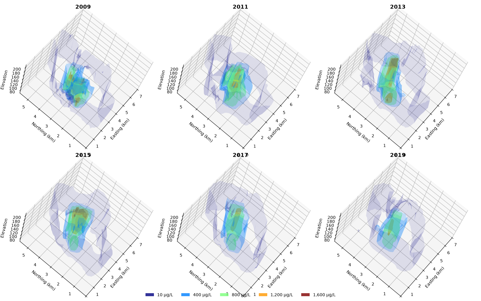
Nested isosurfaces are extracted from each annual concentration volume with marching_cubes() and rendered as Poly3DCollection patches in a 2 × 3 panel (one subplot per snapshot year).

Axes are in local kilometres from the domain’s south-west corner; elevation is preserved in the native unit of the raster files.

Note

Marching cubes assumes a uniform vertical spacing (average layer thickness), which is an approximation for this variable-thickness aquifer. For publication-quality isosurfaces on the true irregular grid, use PyVista.

from skimage.measure import marching_cubes
from mpl_toolkits.mplot3d.art3d import Poly3DCollection
from matplotlib.patches import Patch

avg_dz = float(dz.mean())
z_top  = float(top.mean())

ISO_LEVELS = [10.0, 400.0, 800.0, 1200.0, 1600.0]
ISO_ALPHAS = [0.10, 0.22, 0.45, 0.65, 0.85]
ISO_LABELS = ["10 µg/L", "400 µg/L", "800 µg/L", "1,200 µg/L", "1,600 µg/L"]
_cm = plt.get_cmap("jet", len(ISO_LEVELS))
ISO_COLORS = [_cm(i / (len(ISO_LEVELS) - 1)) for i in range(len(ISO_LEVELS))]

fig, axes = plt.subplots(2, 3, figsize=(16, 10),
                          subplot_kw={"projection": "3d"},
                          tight_layout=True)

for ax, yr in zip(axes.ravel(), KRIGE_YEARS):
    conc = conc_vols[yr]

    for level, color, alpha in zip(ISO_LEVELS, ISO_COLORS, ISO_ALPHAS):
        if conc.max() <= level:
            continue
        try:
            verts, faces, _, _ = marching_cubes(
                conc, level=level,
                spacing=(avg_dz, CELLSIZE, CELLSIZE),
                step_size=2, allow_degenerate=False,
            )
            # Convert marching-cubes index-space verts to km / elevation:
            #   axis 0 = layer (top→bottom, z decreasing)
            #   axis 1 = row   (north→south, local y = NROW*CELLSIZE - offset)
            #   axis 2 = col   (west→east,   local x = offset)
            x_v = verts[:, 2] / 1000
            y_v = (NROW * CELLSIZE - verts[:, 1]) / 1000
            z_v = z_top - verts[:, 0]

            tris = np.stack([x_v[faces], y_v[faces], z_v[faces]], axis=-1)
            ax.add_collection3d(
                Poly3DCollection(tris, alpha=alpha, facecolor=color,
                                 edgecolor="none", linewidth=0)
            )
        except (ValueError, RuntimeError):
            pass

    ax.set_title(str(yr), fontweight="bold", fontsize=13)
    ax.set(xlabel="Easting (km)", ylabel="Northing (km)", zlabel="Elevation")
    ax.set_xlim(0, NCOL * CELLSIZE / 1000)
    ax.set_ylim(0, NROW * CELLSIZE / 1000)
    ax.set_zlim(float(botm.mean()), float(top.mean()))
    ax.view_init(elev=63, azim=-161, roll=-22),

legend_handles = [
    Patch(facecolor=c, alpha=0.8, label=lbl)
    for c, lbl in zip(ISO_COLORS, ISO_LABELS)
]
fig.legend(handles=legend_handles, loc="lower center", ncol=5,
           frameon=False, fontsize=10)
plt.show()