Nested anisotropic variogram fitting from 2-D SGSIM

This example generates several unconditional 2-D Gaussian random fields from a known nested anisotropic variogram, estimates the anisotropy angle from a pooled empirical cloud, and then fits the two generating components to directional bins calculated at that estimated orientation.

The generating model contains:

• a short-range spherical component,

• a longer-range exponential component,

• a shared 2:1 geometric anisotropy at azimuth 30 degrees,

• no nugget, so the example concentrates on nested spatial scales.

Unlike an exact synthetic-curve unit test, empirical variograms from finite random fields contain sampling variation. The fitted values should therefore be interpreted as approximate recovery, not exact equality with the inputs. Pooling several realizations makes the two spatial scales easier to identify.

import matplotlib.pyplot as plt
import numpy as np
import pandas as pd

from krigekit import Kriging, VariogramModel
from krigekit.variogram import estimate_aniso_angle, plot_vgm_map, raw_vgm

Define the nested generating model

AZIMUTH = 30.0
ANIS1 = 0.5
SEED = 2026
NSIM = 16

TRUE_COMPONENTS = [
    dict(
        vtype="sph",
        nugget=0.0,
        sill=0.40,
        a_major=8.0,
        a_minor1=4.0,
        azimuth=AZIMUTH,
        name="short spherical",
    ),
    dict(
        vtype="exp",
        nugget=0.0,
        sill=0.80,
        a_major=30.0,
        a_minor1=15.0,
        azimuth=AZIMUTH,
        name="long exponential",
    ),
]

true_model = VariogramModel()
for spec in TRUE_COMPONENTS:
    true_model.set_vgm(**spec)

Generate unconditional SGSIM realizations

Empty observations request an unconditional simulation. Search anisotropy is set equal to the model anisotropy so previously simulated nodes are selected in the same geometric frame as the covariance model.

axis = np.arange(0.0, 100.0, 2.0)
gx, gy = np.meshgrid(axis, axis, indexing="xy")
grid = np.column_stack([gx.ravel(), gy.ravel()])

simulator = Kriging(ndim=2, nvar=1, nsim=NSIM, seed=SEED)
simulator.set_obs(
    ivar=1,
    coord=np.empty((0, 2)),
    value=np.empty(0),
)
simulator.set_grid(coord=grid)
for spec in TRUE_COMPONENTS:
    engine_spec = {key: value for key, value in spec.items() if key != "name"}
    simulator.set_vgm(ivar=1, jvar=1, **engine_spec)
simulator.set_sim()
simulator.set_search(ivar=1, anis1=ANIS1, azimuth=AZIMUTH, nmax=48)
simulator.solve()

simulations = np.asarray(simulator.get_results()[0])
if simulations.ndim == 1:
    simulations = simulations[:, None]

print(
    f"Generated {simulations.shape[1]} realizations on "
    f"{simulations.shape[0]} grid nodes."
)
print(
    "Per-realization variance:",
    np.round(simulations.var(axis=0), 3),
)

Generated 16 realizations on 2500 grid nodes.
Per-realization variance: [1.52  1.221 1.092 1.204 1.095 1.364 1.442 1.251 1.196 0.977 1.163 1.224
 1.165 1.283 1.43  1.151]

Inspect one realization

fig, ax = plt.subplots(figsize=(7.0, 5.5), layout="constrained")
image = ax.imshow(
    simulations[:, 0].reshape(len(axis), len(axis)),
    origin="lower",
    extent=[axis.min(), axis.max(), axis.min(), axis.max()],
    cmap="coolwarm",
)
fig.colorbar(image, ax=ax, label="simulated value")
ax.set(
    xlabel="X",
    ylabel="Y (North)",
    title="One unconditional nested anisotropic realization",
)

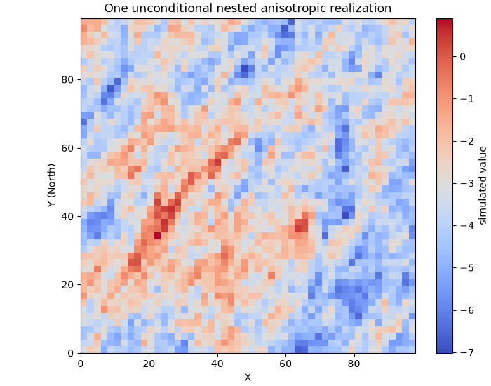
[Text(0.5, 18.055888888888887, 'X'), Text(81.66177586805559, 0.5, 'Y (North)'), Text(0.5, 1.0, 'One unconditional nested anisotropic realization')]

Pool the empirical clouds and estimate the orientation

Holding every pair from every realization would be unnecessarily expensive. Instead, each raw cloud is averaged onto its signed lag cells, then matching cells are pooled across realizations with pair-count weights. The angle estimator uses this compact denoised cloud.

lag_cell_tables = []
for realization in range(simulations.shape[1]):
    raw = raw_vgm(
        grid,
        simulations[:, realization],
        cutoff=62.0,
        calc_angle=True,
        n_jobs=None,
        verbose=False,
    )
    cells = (
        raw
        .groupby(["d0", "d1"], sort=False)
        .agg(
            distance=("distance", "mean"),
            variogram=("variogram", "mean"),
            count=("variogram", "size"),
            angle_h=("angle_h", "mean"),
        )
        .reset_index()
    )
    cells["weighted_variogram"] = cells["count"] * cells["variogram"]
    lag_cell_tables.append(cells)

lag_cells = pd.concat(lag_cell_tables, ignore_index=True)
pooled_cloud = (
    lag_cells
    .groupby(["d0", "d1"], sort=False)
    .agg(
        distance=("distance", "mean"),
        weighted_variogram=("weighted_variogram", "sum"),
        count=("count", "sum"),
        angle_h=("angle_h", "mean"),
    )
    .reset_index()
)
pooled_cloud["variogram"] = (
    pooled_cloud["weighted_variogram"] / pooled_cloud["count"]
)
pooled_cloud = pooled_cloud.drop(columns="weighted_variogram")

# On a regular grid, a radius that is too small is dominated by axis-aligned
# lattice lags. This radius includes several off-axis lag cells while remaining
# focused on the shorter spatial scale.
ANGLE_R_MAX = 12.1
(estimated_azimuth,), (pca_anis1,) = estimate_aniso_angle(
    pooled_cloud,
    r_max=ANGLE_R_MAX,
)


def _axis_difference(angle0, angle1):
    """Smallest difference between two undirected azimuth axes."""
    return abs((angle0 - angle1 + 90.0) % 180.0 - 90.0)


print(
    f"Estimated azimuth = {estimated_azimuth:.2f} degrees "
    f"(true {AZIMUTH:.2f}, axis error "
    f"{_axis_difference(estimated_azimuth, AZIMUTH):.2f} degrees)"
)
print(
    f"PCA spread-ratio estimate = {pca_anis1:.3f}; "
    "the component ranges are fitted below."
)

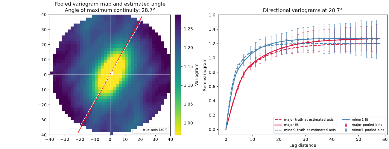
Estimated azimuth = 28.69 degrees (true 30.00, axis error 1.31 degrees)
PCA spread-ratio estimate = 0.693; the component ranges are fitted below.

Calculate directional variograms at the estimated angle

The cloud is recalculated one realization at a time so the full pair tables never accumulate in memory. Directional bins now use the estimated azimuth, not the known generating angle.

directional_tables = []
for realization in range(simulations.shape[1]):
    analysis = VariogramModel()
    analysis.set_obs(grid, simulations[:, realization])
    analysis.set_vgm(
        "sph",
        sill=1.0,
        a_major=10.0,
        a_minor1=5.0,
        azimuth=estimated_azimuth,
    )
    analysis.calc_experimental(
        cutoff=62.0,
        calc_angle=True,
        n_jobs=None,
        verbose=False,
    )
    table = analysis.calc_directional_average(
        h_width=2.0,
        cutoff=58.0,
        angle_tol=12.5,
        robust=False,
    ).copy()
    table["realization"] = realization
    directional_tables.append(table)

directional_all = pd.concat(directional_tables, ignore_index=True)

directional_all["weighted_variogram"] = (
    directional_all["count"] * directional_all["variogram"]
)
pooled = (
    directional_all
    .groupby(["direction", "axis", "lag"], observed=True, sort=True)
    .agg(
        weighted_variogram=("weighted_variogram", "sum"),
        count=("count", "sum"),
        between_realization_std=("variogram", "std"),
    )
    .reset_index()
)
pooled["variogram"] = pooled["weighted_variogram"] / pooled["count"]
pooled = pooled.drop(columns="weighted_variogram")

# Balance the two axes in the fit. Without this normalization, the axis with
# more accepted pairs can dominate the least-squares objective.
pooled["axis_weight"] = (
    pooled["count"]
    / pooled.groupby("axis", observed=True)["count"].transform("sum")
)

Fit a two-component anisotropic model

The orientation is fixed at the pooled-cloud estimate. The fit estimates each component’s sill, major range, and minor range:

sill_short, major_short, minor_short, sill_long, major_long, minor_long.

fitted_model = VariogramModel()
fitted_model.set_vgm(
    "sph",
    nugget=0.0,
    sill=0.30,
    a_major=7.0,
    a_minor1=3.5,
    azimuth=estimated_azimuth,
    name="short spherical",
)
fitted_model.set_vgm(
    "exp",
    sill=0.70,
    a_major=24.0,
    a_minor1=12.0,
    azimuth=estimated_azimuth,
    name="long exponential",
)

fit = fitted_model.fit_anisotropy(
    pooled,
    p0=(0.30, 7.0, 3.5, 0.70, 24.0, 12.0),
    bounds=(
        [0.01, 2.0, 1.0, 0.05, 12.0, 5.0],
        [1.50, 16.0, 10.0, 2.00, 70.0, 40.0],
    ),
    weight_col="axis_weight",
    inplace=True,
    fit_nugget=False,
    maxfev=50000,
)

fitted = fit.target

comparison = []
for true_component, fitted_component in zip(
    true_model.structure.components,
    fitted.structure.components,
):
    comparison.append({
        "component": true_component.display_name,
        "true_sill": true_component.sill,
        "fitted_sill": fitted_component.sill,
        "true_major": true_component.a_major,
        "fitted_major": fitted_component.a_major,
        "true_minor": true_component.a_minor1,
        "fitted_minor": fitted_component.a_minor1,
    })

comparison = pd.DataFrame(comparison)
print("\nTrue and fitted nested components:")
print(comparison.to_string(index=False, float_format=lambda value: f"{value:7.3f}"))

True and fitted nested components:
       component  true_sill  fitted_sill  true_major  fitted_major  true_minor  fitted_minor
 short spherical      0.400        0.443       8.000         8.784       4.000         4.404
long exponential      0.800        0.829      30.000        34.965      15.000        21.483

Compare empirical bins, generating curves, and fitted curves

angle = np.deg2rad(estimated_azimuth)
directions = {
    "major": np.array([np.sin(angle), np.cos(angle)]),
    "minor1": np.array([np.cos(angle), -np.sin(angle)]),
}
colors = {"major": "crimson", "minor1": "steelblue"}

fig, axes = plt.subplots(1, 2, figsize=(13.0, 5.0), layout="constrained")

plot_vgm_map(
    pooled_cloud,
    ax=axes[0],
    cutoff=40.0,
    dx=2.0,
    dy=2.0,
    angle_aniso=estimated_azimuth,
    ellipse_aniso=None,
    title="Pooled variogram map and estimated angle",
)
rm = 42.0
true_x = rm * np.sin(np.deg2rad(AZIMUTH))
true_y = rm * np.cos(np.deg2rad(AZIMUTH))
axes[0].plot(
    [true_x, -true_x],
    [true_y, -true_y],
    color="white",
    linestyle="--",
    linewidth=1.5,
    label=f"true axis ({AZIMUTH:.0f}°)",
    zorder=25,
)
axes[0].legend(loc="lower right", fontsize=8)

for axis_name in ("major", "minor1"):
    subset = pooled.loc[pooled["axis"] == axis_name]
    axes[1].errorbar(
        subset["lag"],
        subset["variogram"],
        yerr=subset["between_realization_std"],
        fmt="o",
        ms=4,
        capsize=2,
        alpha=0.65,
        color=colors[axis_name],
        label=f"{axis_name} pooled bins",
    )

    h = np.linspace(0.0, 58.0, 300)
    coord0 = np.zeros((len(h), 2))
    coord1 = directions[axis_name] * h[:, None]
    axes[1].plot(
        h,
        true_model.calc_variogram(coord0, coord1),
        color=colors[axis_name],
        linestyle="--",
        linewidth=2.0,
        label=f"{axis_name} truth at estimated axis",
    )
    axes[1].plot(
        h,
        fitted.calc_variogram(coord0, coord1),
        color=colors[axis_name],
        linewidth=2.0,
        label=f"{axis_name} fit",
    )

axes[1].set(
    xlabel="Lag distance",
    ylabel="Semivariogram",
    title=f"Directional variograms at {estimated_azimuth:.1f}°",
)
axes[1].legend(fontsize=8, ncol=2)

plt.show()